Thresholding#
import zarr
import zarr.storage
import fsspec
import numpy as np
import xarray as xr
import matplotlib.pyplot as plt
from matplotlib.colors import LogNorm
from scipy.signal import stft
from scipy.signal import find_peaks
from collections import defaultdict
# List of shot IDs
shot_ids = [23447, 30005, 30021, 30421]  # Add more as needed

# S3 endpoint
endpoint = "https://s3.echo.stfc.ac.uk"
fs = fsspec.filesystem(
    protocol='simplecache',
    target_protocol="s3",
    target_options=dict(anon=True, endpoint_url=endpoint)
)
store_list = []
zgroup_list = []
# Loop through each shot ID
for shot_id in shot_ids:
    url = f"s3://mast/level2/shots/{shot_id}.zarr"

    store = zarr.storage.FSStore(fs=fs, url=url)
    store_list.append(store)
    # open or download the Zarr group
    try:
        zgroup_list.append(zarr.open(store, mode='r'))
        print(f"Loaded shot ID {shot_id}")
        # Do something with zgroup here, like listing arrays:
        # print(list(zgroup.array_keys()))
    except Exception as e:
        print(f"Failed to load shot ID {shot_id}: {e}")
Loaded shot ID 23447
Loaded shot ID 30005
Loaded shot ID 30021
Loaded shot ID 30421
# for store in zgroup:
#     root = zarr.open_group(store, mode='r')
mirnov = [xr.open_zarr(store, group="magnetics") for store in store_list]
mirnov[0]
<xarray.Dataset> Size: 32MB
Dimensions: (b_field_pol_probe_cc_channel: 5,
time_mirnov: 261200,
b_field_pol_probe_ccbv_channel: 40,
time: 2612,
b_field_pol_probe_obr_channel: 18,
b_field_pol_probe_obv_channel: 18,
b_field_pol_probe_omv_channel: 3,
b_field_tor_probe_cc_channel: 3,
b_field_tor_probe_saddle_field_channel: 12,
time_saddle: 26120,
b_field_tor_probe_saddle_voltage_channel: 12,
flux_loop_channel: 15)
Coordinates:
* b_field_pol_probe_cc_channel (b_field_pol_probe_cc_channel) <U13 260B ...
* b_field_pol_probe_ccbv_channel (b_field_pol_probe_ccbv_channel) <U10 2kB ...
* b_field_pol_probe_obr_channel (b_field_pol_probe_obr_channel) <U9 648B ...
* b_field_pol_probe_obv_channel (b_field_pol_probe_obv_channel) <U9 648B ...
* b_field_pol_probe_omv_channel (b_field_pol_probe_omv_channel) <U11 132B ...
* b_field_tor_probe_cc_channel (b_field_tor_probe_cc_channel) <U13 156B ...
* b_field_tor_probe_saddle_field_channel (b_field_tor_probe_saddle_field_channel) <U11 528B ...
* b_field_tor_probe_saddle_voltage_channel (b_field_tor_probe_saddle_voltage_channel) <U15 720B ...
* flux_loop_channel (flux_loop_channel) <U12 720B '...
* time (time) float64 21kB -0.099 ... ...
* time_mirnov (time_mirnov) float64 2MB -0.09...
* time_saddle (time_saddle) float64 209kB -0....
Data variables:
b_field_pol_probe_cc_field (b_field_pol_probe_cc_channel, time_mirnov) float64 10MB ...
b_field_pol_probe_ccbv_field (b_field_pol_probe_ccbv_channel, time) float64 836kB ...
b_field_pol_probe_obr_field (b_field_pol_probe_obr_channel, time) float64 376kB ...
b_field_pol_probe_obv_field (b_field_pol_probe_obv_channel, time) float64 376kB ...
b_field_pol_probe_omv_voltage (b_field_pol_probe_omv_channel, time_mirnov) float64 6MB ...
b_field_tor_probe_cc_field (b_field_tor_probe_cc_channel, time_mirnov) float64 6MB ...
b_field_tor_probe_saddle_field (b_field_tor_probe_saddle_field_channel, time_saddle) float64 3MB ...
b_field_tor_probe_saddle_voltage (b_field_tor_probe_saddle_voltage_channel, time_saddle) float64 3MB ...
flux_loop_flux (flux_loop_channel, time) float64 313kB ...
ip (time) float64 21kB ...
Attributes:
description:
imas: magnetics
label: Plasma Current
name: magnetics
uda_name: AMC_PLASMA CURRENT
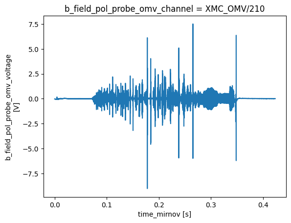
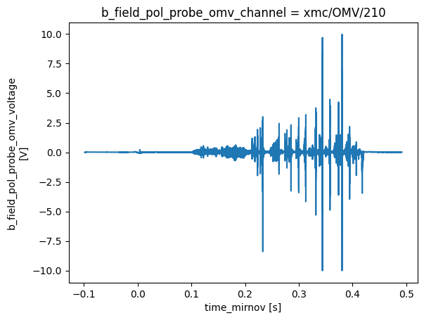
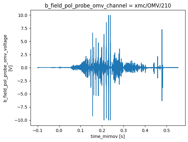
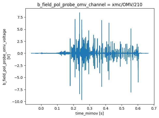
units: A# Extract the DataArrays
ds_list = [m['b_field_pol_probe_omv_voltage'].isel(b_field_pol_probe_omv_channel=1) for m in mirnov]
# Plot all in one figure
for i, ds in enumerate(ds_list):
plt.figure(i)
ds.plot(label=f"Shot {i}")
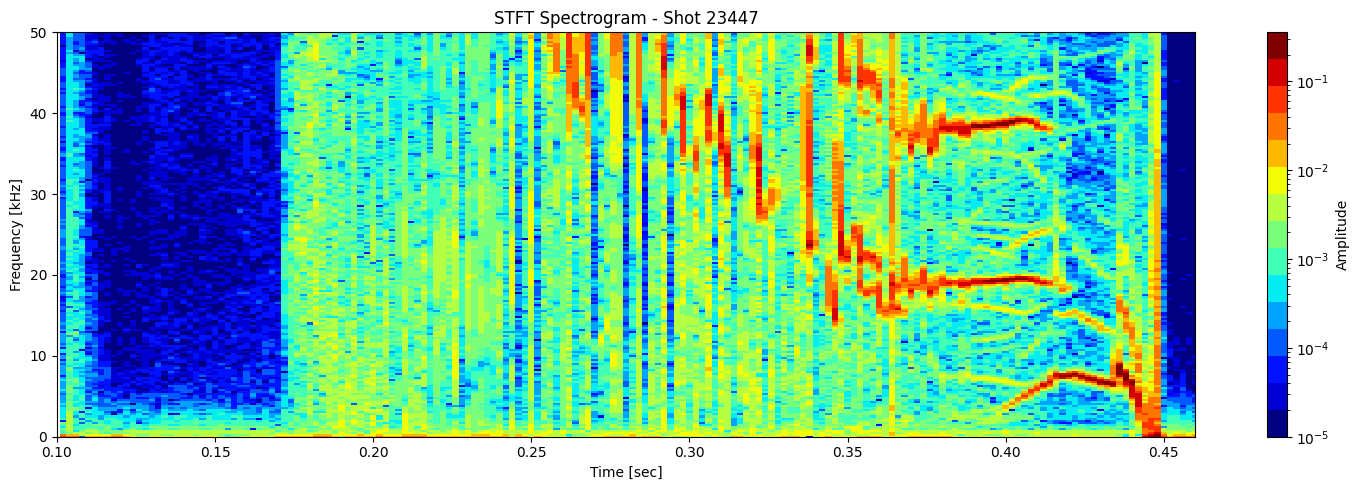
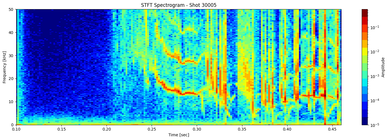
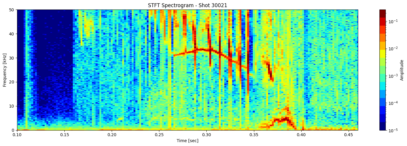
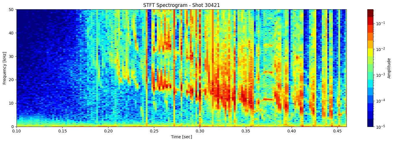
Short-Time Fourier Transform (STFT)#
def plot_stft_spectrogram(    ds,    shot_id=None,    nperseg=2000,    nfft=2000,    tmin=0.1,    tmax=0.46,    fmax_kHz=50,    cmap='jet'):
    """
    Plot STFT spectrogram for a given xarray DataArray `ds`.

    Parameters:
    - ds: xarray.DataArray with a 'time_mirnov' coordinate.
    - shot_id: Optional shot ID for labeling.
    - nperseg: Number of points per STFT segment.
    - nfft: Number of FFT points.
    - tmin, tmax: Time range to display (seconds).
    - fmax_kHz: Max frequency to display (kHz).
    - cmap: Colormap name.
    """
    sample_rate = 1 / float(ds.time_mirnov[1] - ds.time_mirnov[0])
    f, t, Zxx = stft(ds.values, fs=int(sample_rate), nperseg=nperseg, nfft=nfft)

    fig, ax = plt.subplots(figsize=(15, 5))
    cax = ax.pcolormesh(
        t, f / 1000, np.abs(Zxx),
        shading='nearest',
        cmap=plt.get_cmap(cmap, 15),
        norm=LogNorm(vmin=1e-5)
    )
    ax.set_ylim(0, fmax_kHz)
    ax.set_xlim(tmin, tmax)
    ax.set_ylabel('Frequency [kHz]')
    ax.set_xlabel('Time [sec]')
    title = f"STFT Spectrogram"
    if shot_id is not None:
        title += f" - Shot {shot_id}"
    ax.set_title(title)
    plt.colorbar(cax, ax=ax, label='Amplitude')
    plt.tight_layout()
[plot_stft_spectrogram(ds_list[i], shot_ids[i]) for i in range(len(ds_list))]
[None, None, None, None]
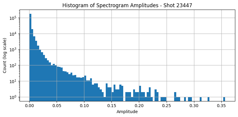
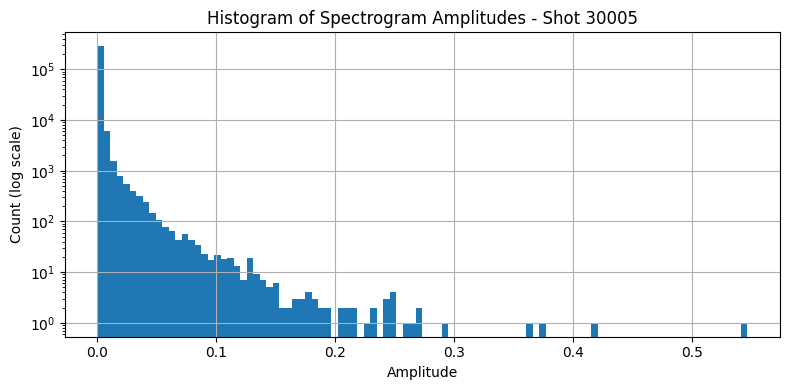
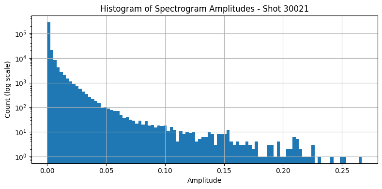
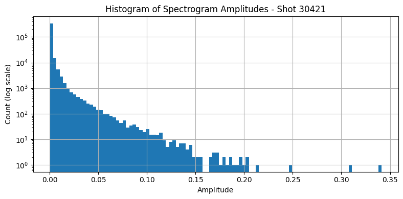
Inspect amplitude distribution#
def plot_stft_histogram(    ds,    shot_id=None,    nperseg=2000,    nfft=2000,    bins=100
):
    """
    Plot a histogram of the absolute STFT amplitude values.

    Parameters:
    - ds: xarray.DataArray with a 'time_mirnov' coordinate.
    - shot_id: Optional shot ID for labeling.
    - nperseg: Number of points per STFT segment.
    - nfft: Number of FFT points.
    - bins: Number of histogram bins.
    """
    sample_rate = 1 / float(ds.time_mirnov[1] - ds.time_mirnov[0])
    f, t, Zxx = stft(ds.values, fs=int(sample_rate), nperseg=nperseg, nfft=nfft)

    plt.figure(figsize=(8, 4))
    plt.hist(np.abs(Zxx.flatten()), bins=bins, log=True)
    plt.xlabel('Amplitude')
    plt.ylabel('Count (log scale)')
    title = 'Histogram of Spectrogram Amplitudes'
    if shot_id is not None:
        title += f" - Shot {shot_id}"
    plt.title(title)
    plt.grid(True)
    plt.tight_layout()
    return f, t, Zxx
f_list, t_list, Zxx_list =  [], [], []
for i, ds in enumerate(ds_list):
    f, t, Zxx = plot_stft_histogram(ds_list[i], shot_ids[i])
    f_list.append(f)
    t_list.append(t)
    Zxx_list.append(Zxx)

#[plot_stft_histogram(ds_list[i], shot_ids[i]) for i in range(len(ds_list))]
def visualise_thresholded_spectrogram(t, f, binary_mask):
    """
    Visualise the binary mask of the spectrogram.
    """
    fig, ax = plt.subplots(figsize=(15, 5))
    cax = ax.pcolormesh(t, f/1000, binary_mask, shading='nearest', cmap='gray_r')
    #ax.set_ylim(0, 50)
    #ax.set_xlim(0.1, 0.46)
    ax.set_title(f'Shot {shot_id}, Binary Thresholded Modes')
    ax.set_ylabel('Frequency [kHz]')
    ax.set_xlabel('Time [sec]')
    plt.colorbar(cax, ax=ax, label='Mode presence (binary)')
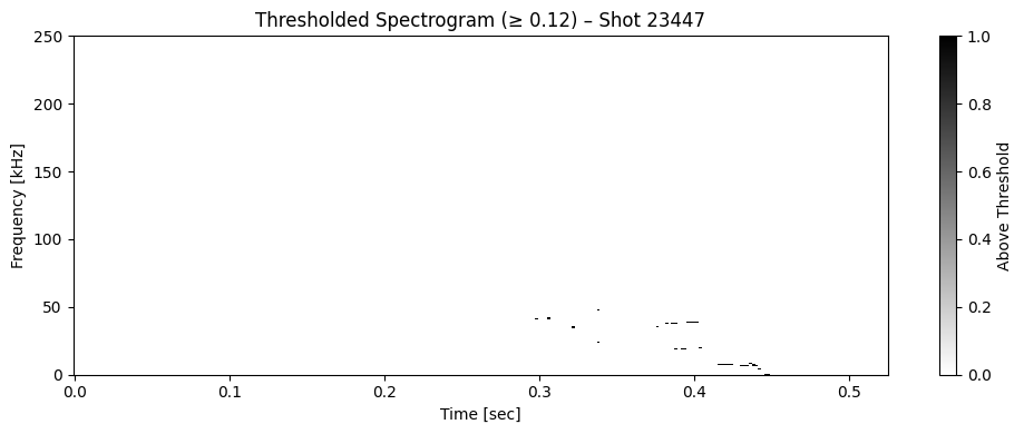
def plot_thresholded_spectrogram(t, f, Zxx, threshold, shot_id=None, cmap='gray_r'):
    """
    Plot a binary spectrogram mask after applying an amplitude threshold.

    Parameters:
    - t: 1D time array (from STFT)
    - f: 1D frequency array (from STFT)
    - Zxx: 2D complex STFT result
    - threshold: Amplitude threshold for binary mask
    - shot_id: Optional shot ID for labeling
    - cmap: Colormap for visualization (default: 'gray_r')
    """
    # Compute binary mask
    binary_mask = np.abs(Zxx) >= threshold

    # Plot
    plt.figure(figsize=(10, 4))
    plt.pcolormesh(t, f / 1000, binary_mask, shading='nearest', cmap=cmap)
    plt.xlabel('Time [sec]')
    plt.ylabel('Frequency [kHz]')
    plt.title(f'Thresholded Spectrogram (≥ {threshold})' + (f' – Shot {shot_id}' if shot_id else ''))
    plt.colorbar(label='Above Threshold')
    plt.tight_layout()
# Define a threshold (e.g., percentile-based threshold)
threshold = 0.12 #np.percentile(np.abs(Zxx), 50)  # top 5% amplitudes

[plot_thresholded_spectrogram(t_list[0], f_list[0], Zxx_list[0], threshold, shot_ids[0]) for i in range(len(ds_list))]
[None, None, None, None]
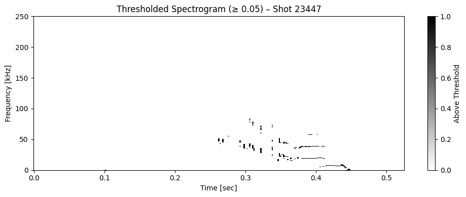
# Define a threshold (e.g., percentile-based threshold)
threshold = 0.05 #np.percentile(np.abs(Zxx), 50)  # top 5% amplitudes

[plot_thresholded_spectrogram(t_list[0], f_list[0], Zxx_list[0], threshold, shot_ids[0]) for i in range(len(ds_list))]
[None, None, None, None]
# Define a threshold (e.g., percentile-based threshold)
threshold = 0.01 #np.percentile(np.abs(Zxx), 50)  # top 5% amplitudes

[plot_thresholded_spectrogram(t_list[0], f_list[0], Zxx_list[0], threshold, shot_ids[0]) for i in range(len(ds_list))]
[None, None, None, None]
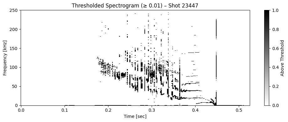
Playing with the plots#
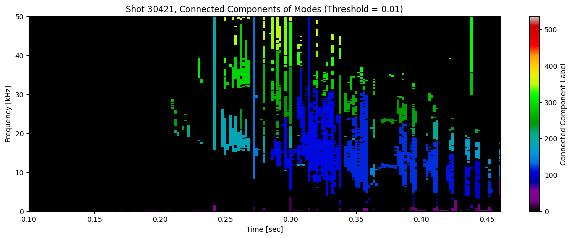
from scipy.ndimage import label, find_objects

# Binary mask at threshold 0.01
threshold = 0.01
binary_mask = np.abs(Zxx) >= threshold
# Label connected regions
labeled_array, num_features = label(binary_mask)

print(f'Number of connected mode regions identified: {num_features}')
Number of connected mode regions identified: 537
fig, ax = plt.subplots(figsize=(15, 5))
cax = ax.pcolormesh(t, f/1000, labeled_array, shading='nearest', cmap="nipy_spectral")#plt.get_cmap('nipy_spectral', 50))
ax.set_ylim(0, 50)
ax.set_xlim(0.1, 0.46)
ax.set_title(f'Shot {shot_id}, Connected Components of Modes (Threshold = {threshold})')
ax.set_ylabel('Frequency [kHz]')
ax.set_xlabel('Time [sec]')
plt.colorbar(cax, ax=ax, label='Connected Component Label')
plt.show()