Burgers equation — 1D space and time¶

Open File → Examples → 1D examples → Burgers — 1D + time. This uses the continuous-time viscous Burgers problem presented by Raissi, Perdikaris and Karniadakis in the original PINN work. The authors' problem description is the setup reference; no TensorFlow source or reference dataset is copied.

u_t + u*u_x - nu*u_xx = 0
nu = 0.01/pi
x in [-1, 1], t in [0, 1]
u(x, 0) = -sin(pi*x)
u(-1, t) = u(1, t) = 0

The problem is 1D in space, although its network has two inputs (x,t). It is a continuous space–time PINN; it does not advance the solution through numerical timesteps.

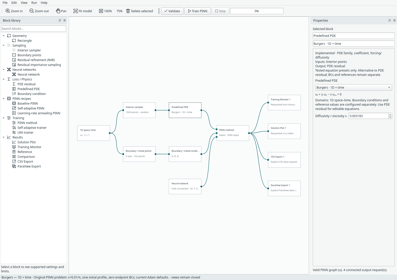
The Burgers example has an explicit time-dependent PDE and space–time domain

Domain, samples and initial condition¶

The existing domain block has a 1D space–time option. Set spatial bounds with x minimum/maximum and physical-time bounds with t start/end. Interior points sample the (x,t) slab. The boundary/initial sampler produces:

Set	Coordinates	Default condition
Left boundary	`x=-1`, sampled `t`	`u=0`
Right boundary	`x=1`, sampled `t`	`u=0`
Initial	sampled `x`, `t=0`	`u=-sin(pi*x)`

There is no final-time condition. The initial profile must agree with the spatial boundary values at its endpoints. Its named training loss is initial, shown separately from PDE and spatial BC curves in the Training Monitor.

The initial set reuses the sampler's internal bottom storage key; the UI labels it initial (t start). top settings retained from rectangular models are inactive. For save-format compatibility, y_min/y_max store the time bounds; the UI and exported coordinates call them t.

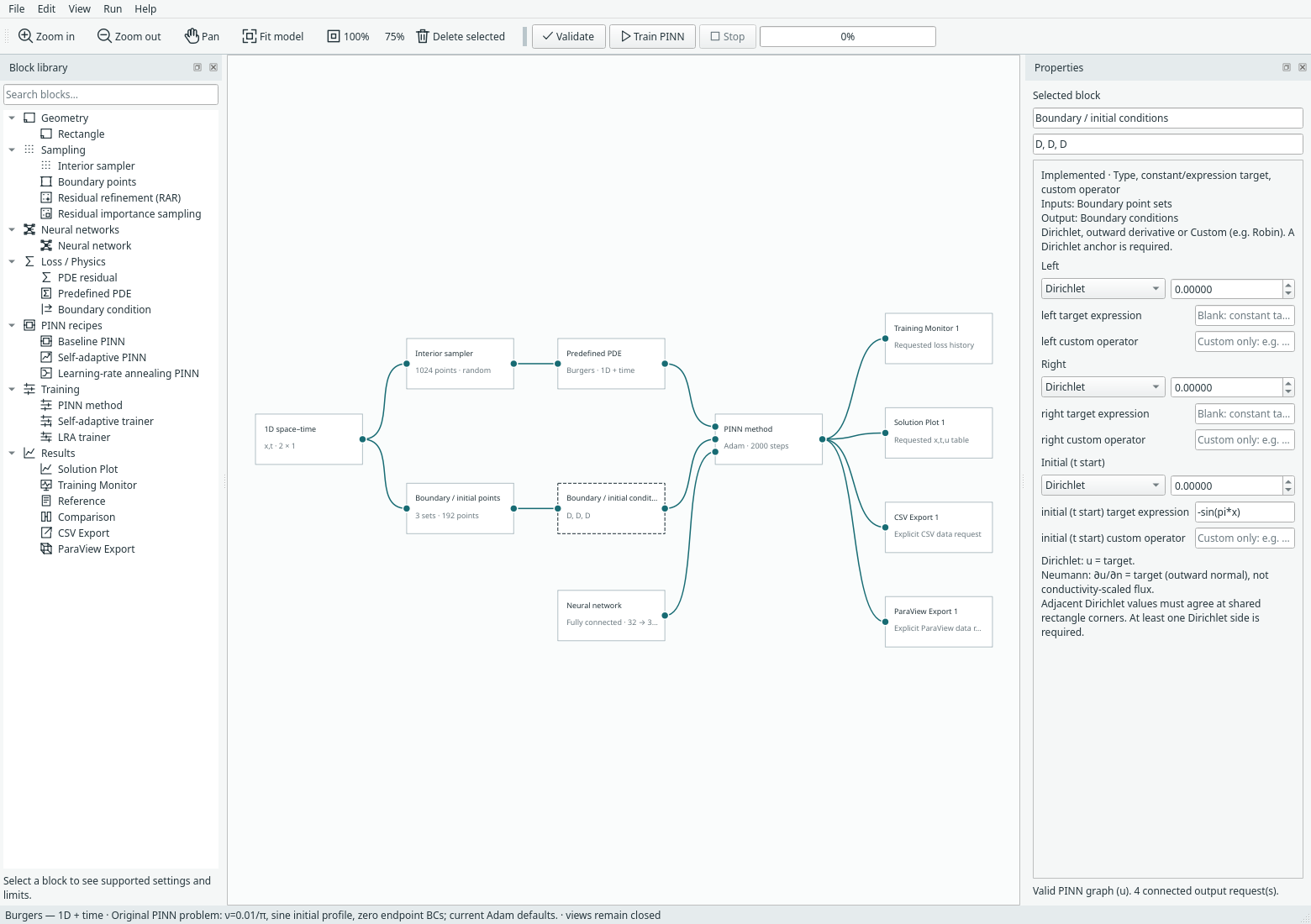
Initial conditions are assigned independently of the two spatial boundary traces

PDE and network¶

The Burgers · 1D + time preset exposes viscosity and constructs:

D(u,t) + u*D(u,x) - nu*D(D(u,x),x)

It requires positive viscosity and a space–time domain. Restricted expressions use x,t, not x,y, for this domain. D(u,t) differentiates physical time; laplace(u) differentiates spatial coordinates only. Scalar expressions also support the configured nu. Existing spatial models retain their x / x,y coordinate meanings and reject a time derivative.

The example defaults to 1,024 seeded random interior points, 64 samples on each of the three constraint sets, a tanh network with three 32-neuron hidden layers, and 2,000 Adam updates at learning rate 0.001. These are editable Margam defaults, not a reproduction of the paper's architecture, training budget, optimiser schedule or reported accuracy. The original paper's pooled initial/boundary data loss is represented here using separate named means with existing set weights.

Baseline, SA-PINN and LRA trainers work with this problem. RAR and importance sampling act on (x,t) candidates using their existing compatibility rules. Integral loss uses space–time measure for the PDE, time length for left/right traces and spatial length for the initial profile. The all-sides hard-Dirichlet transform is rejected because it would also constrain the final time.

Results and export¶

Training Monitor, Solution Plot, CSV Export and ParaView Export blocks are wired in this example; their views remain closed until requested. Training creates no export files. The solution block opens an x,t,u table, reusing the current table widget; this change adds no field heatmap or automatic figure pane.

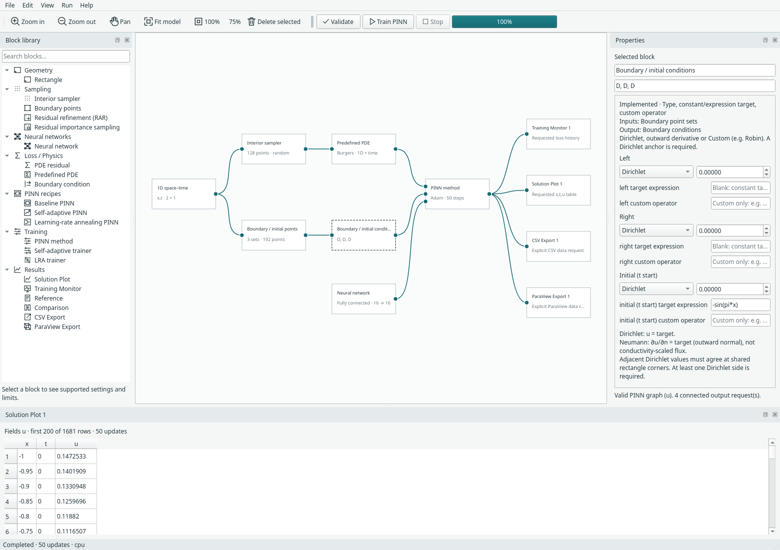
The optional Burgers solution view shows coordinates and predicted values

No Reference or Comparison block is added: the sine initial profile is not a reference solution at later times. No reference/error metric is invented. Users can explicitly supply compatible mapped reference values or a valid expression.

CSV exports use columns x,t,u. The ParaView block writes a .pvd series with one spatial line .vti per physical evaluation time. With evaluation resolution N, there are N spatial points at each of N times, including the initial/final bounds. Open the PVD in ParaView and press Play. Keep its generated frame directory beside the index file. Time is stored as frame timestamps, never as a second spatial coordinate or as training-update numbers.

Saved models and run archives retain the space–time domain, IC, network and checkpoint. Earlier model versions remain readable. Compact recipe expansion/collapse retains this same problem configuration.

Verification and reproducible commands¶

From the repository root and existing environment:

python -m examples.burgers
python -m examples.burgers --steps 100 --export results/burgers.pvd
python -m unittest discover -s tests -p 'test_burgers*.py' -v
python -m examples.capture_burgers --overwrite

The CPU workflow record records 100 updates, finite losses, exact checkpoint continuation and nine correctly timestamped line frames. Tests separately check analytic derivatives, nonlinear residual terms, viscosity, initial/boundary coordinates, absence of final-time constraints, method and sampler combinations, CSV headings and archive/UI behaviour. This is software correctness evidence; the shock profile has not been validated against the paper's reference data and no paper-accuracy claim is made.