Geometry documents with Jorvik¶

Add Geometry → Jorvik geometry when you want to prepare CAD-derived samples in a separate editor. Simple rectangles still work directly in Margam. Jorvik owns geometry, boundary regions and sampling; Margam owns PDEs, boundary operators, networks and training. No 3D viewport is embedded in Margam.

Install the editor¶

Install Jorvik into the existing root environment. For sibling local checkouts:

uv pip install --python .venv/bin/python ../Jorvik

Use a Jorvik version providing create_empty_project and command-line opening of .jorvik files. Both applications currently require PySide6 6.12.0. The optional Margam geometry extra declares the NetCDF reader dependencies, xarray and SciPy; installing Jorvik supplies those too. Margam's ordinary built-in domains do not require Jorvik. Importing a model never launches the external editor automatically.

Edit, save and apply¶

1. Add Jorvik geometry from the block library. It creates an empty .jorvik document in the current project's working folder.
2. Right-click the block → Edit in Jorvik, or double-click it. Import your geometry, define named boundary regions and generate samples there.
3. Save the Jorvik document after generating samples. Margam reads its saved generated datasets and exports domain.nc automatically when the editor closes. No manual export step is needed. It also regenerates the export when you choose Update, so a stale adjacent NetCDF file is not reused.
4. Close Jorvik. Back in Margam, right-click → Update from Jorvik.
5. Review the dataset table. Roles are preselected from Jorvik sampling metadata; boundary names are prefilled from the exported labels and remain editable. Each boundary dataset has its own row. Confirm the coordinate plane, one Interior dataset and one or more Boundary datasets. Ignore is an explicit opt-out, not the default. Boundary names start with a letter, followed by letters, digits, _ or -.
6. Confirm the update. Margam creates or updates Interior data and Boundary data blocks connected to this geometry. Connect their outputs to the PDE and Boundary condition blocks, respectively. Also connect Boundary data to the PDE block's optional boundary input if you want the PDE enforced there. Without that arrow, it is not. Remove the original rectangle/samplers if replacing an existing template; each executable graph has one geometry.
7. Assign the PDE and boundary types/targets in Margam. For result outputs, supply an explicit Evaluation points block; Margam does not fill the geometry's bounding box with evaluation points.

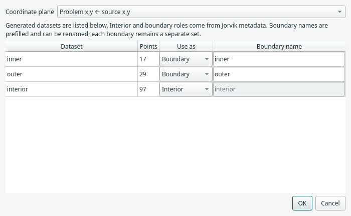
Real Jorvik annulus export: 97 interior points, 17 inner-boundary points and 29 outer-boundary points. Metadata selects the default roles; editable names preserve the exported labels. No PDE or BC type is inferred from a name.

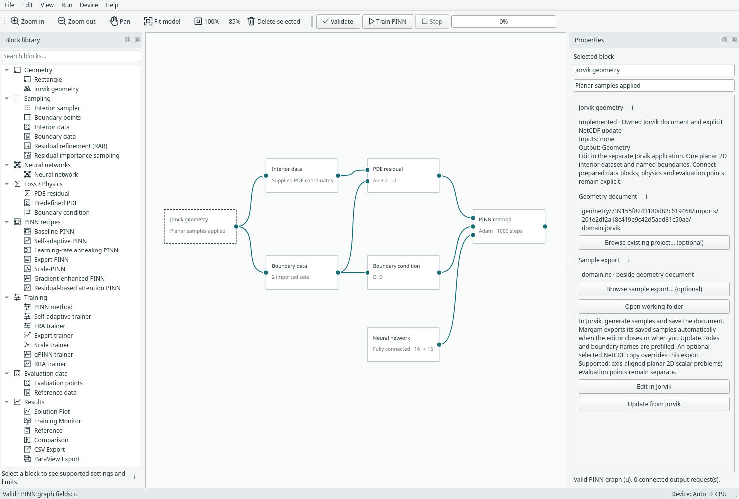
The geometry block opens its document in the external editor. This capture applies a saved annulus document and automatically exports its generated samples.

Optional existing files¶

Both browse buttons are optional. A new block still starts with an empty document and defaults to domain.nc beside it.

• Browse existing project… (optional) accepts .jorvik or legacy .gsproj. Margam validates and copies it into this project's owned files. Editing this copy does not overwrite the original. Choosing a different document requires an explicit sample update before training and resets any custom export selection.
• Browse sample export… (optional) accepts an existing Jorvik .nc file with any filename. Margam validates and copies it into its owned files. Update from Jorvik then uses this selected copy, with the usual dataset-role mapping. Selecting the file alone does not apply its datasets. To pick up later external changes, browse the export again.
• Use export beside geometry document clears the optional export override and restores the adjacent domain.nc default.

Both selections are undoable, survive Save/Save As and recovery, and move with the project companion folder. Cancelling a picker leaves the block unchanged. The named BC sets remain separate for physics assignment and individual loss coefficients in the Boundary condition inspector.

Generated samples and separate boundaries¶

Margam exports samples that already exist in the saved Jorvik document; it does not generate new samples or choose sampling budgets. If the saved document has no generated datasets, Update explains that samples must be generated and saved first. Ungenerated sampling requests are not exported. Export errors leave the last applied snapshot unchanged. There is no silent fallback to an older adjacent NetCDF file.

For four independent rectangle BCs, create and sample four named boundary regions in Jorvik. A single dataset containing all edges remains one set; Margam does not split it or invent names from the entity tags. Multiple interior datasets still require choosing one for this executor. Unknown metadata asks for a role rather than defaulting to Ignore. Previous boundary aliases remain selected by stable ID.

An optional Browse sample export selection bypasses automatic project export: that selected copy is the chosen data source. Use Use export beside geometry document to return to automatically exporting the saved project samples.

Updates and boundary identity¶

Each applied update copies the NetCDF file to an immutable, uniquely named snapshot. Later exports do not change an existing run's training inputs. Applying a new snapshot clears trained results and is undoable. A missing or modified snapshot fails validation rather than silently changing inputs.

Jorvik region IDs preserve boundary assignments when a region's display label changes. Where a dataset has no region ID, its label is the fallback identity; renaming that label is therefore a new identity. The selection dialog remembers previous assignments. Reusing an existing boundary name for a different region is rejected. Removed or renamed assignments are listed for confirmation, and their old physics settings are cleared. Overlapping regions are not merged or deduplicated.

Saving and recovery¶

An unsaved Margam model uses a private temporary folder. First Save copies its owned documents and snapshots to <name>_files beside <name>.margam.json. Save As copies that folder and preserves the original project. File pickers start in Documents (or Documents/Margam if it exists) and remember the last project folder when desktop preferences are enabled. Keep the model and its companion folder together when moving or sharing them; their links are relative. Saving to a different model whose companion folder already exists is refused to avoid merging unrelated project files.

While Jorvik is open, editing, saving, project replacement and closing Margam are blocked. Close Jorvik first, so it cannot continue writing to a folder being moved or deleted. Closing it marks the Margam document modified and exports its saved generated samples. Applying those datasets still requires Update and confirmation. Desktop recovery includes owned files from its last recovery snapshot; recovery is paused during external editing and queued when the editor closes. Discard removes temporary working files, not saved project folders.

Current scope¶

The first integration supports steady planar 2D scalar problems, one interior point set and named edge boundaries. Choose XY, XZ or YZ explicitly; all selected points must lie on the same axis-aligned plane. Both chosen coordinates must have nonzero extent. Verified planar outward conormals are preserved; missing normals are allowed for Dirichlet constraints but must be supplied for normal-dependent operators. No direction is inferred from the coordinate bounding box.

NetCDF datasets can have independent row counts. The reader supports Jorvik's sample schema version 2 and NetCDF3 export, with a 64 MiB file limit, at most 100000 interior rows and 100000 boundary rows in total. Units remain those of the source geometry; no unit conversion is performed. Prepared-domain method limits still apply: no automatic RAR/importance candidate generation, integral quadrature, or Expert/Scale fresh sampling on unknown domains. Copy/paste of owned geometry and owned data blocks is currently disabled. Existing linked CSV/NPZ inputs are unchanged; new imports can optionally be copied into the project using File handling in their mapping dialogs.

This integration does not import arbitrary 3D volumes, rotated planes, mesh cells, PDE definitions, BC targets or evaluation datasets automatically.

Reproduce the interchange check¶

CUDA_VISIBLE_DEVICES='' .venv/bin/python -m examples.jorvik_exchange --output assets/benchmarks/jorvik-exchange.json
QT_QPA_PLATFORM=offscreen .venv/bin/python -m examples.capture_jorvik --overwrite

The recorded CPU check generates an annulus through Jorvik/Gmsh, checks inner/outer normal orientation, trains four baseline updates from the NetCDF data and compares uninterrupted training with 2+2 checkpoint continuation. It is an interchange/lifecycle check, not evidence of solution accuracy. Additional automated UI checks cover document creation, editor launch arguments, locking, update/undo, failed update preservation, first Save, Save As, relocation and changed-snapshot rejection.

Walk through a complete project¶

This example checks the complete desktop workflow with a curved annulus rather than a rectangle. It uses 97 interior, 17 inner-edge and 29 outer-edge samples. The equation is Laplace, with inner Dirichlet u = 0 and outer Neumann ∂u/∂n = 1. The known field u = log(2r) checks the imported operators and normal directions; the short training run is not an accuracy benchmark.

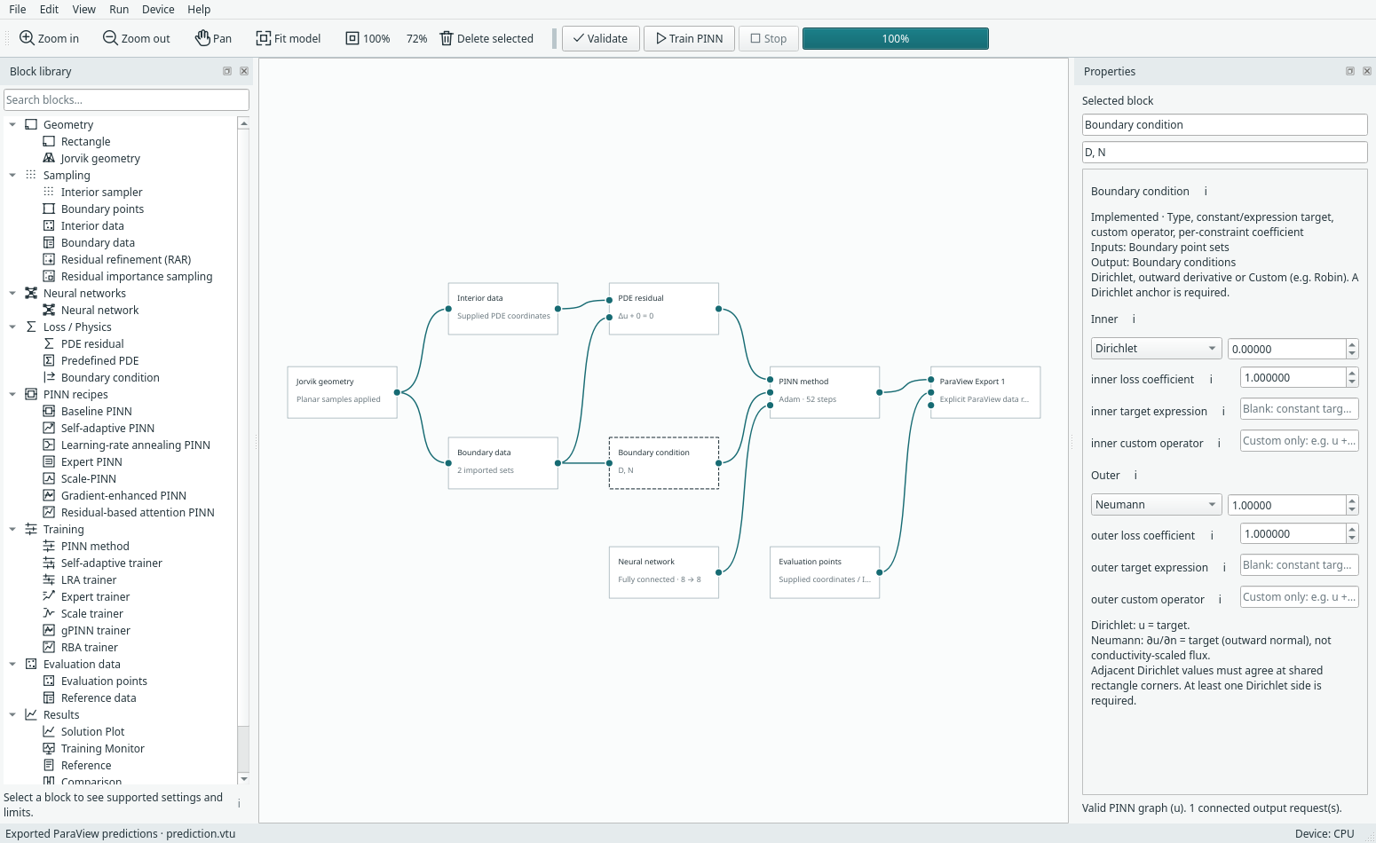
1. Create/sample the annulus in Jorvik, save and apply its datasets as described above. Keep the inner and outer names.
2. Connect Interior data → PDE residual, Boundary data → PDE residual (optional boundary input), and Boundary data → Boundary condition. This graph uses all 143 PDE rows while retaining independent BC losses.
3. Set source to zero. In Boundary condition, set inner Dirichlet value 0 and outer Neumann value 1. Neumann means outward derivative, not a conductivity-scaled flux. Set the trainer's overall boundary weight to 3 if following this check. Each boundary also has its own loss coefficient, default 1. For example, inner 2 and outer 0.5 give effective fixed weights 3 and 0.75 with overall BC weight 3 and two constraints; other terms are not renormalized.
4. Add Evaluation points and map an explicit CSV with columns id,x,y. For example, use probe-C,0.75,0, probe-A,0,0.6, probe-B,-0.8,0. Connect Evaluation points and PINN method to ParaView Export. Evaluation points are independent of training samples; no bounding-box grid is generated.
5. Save the model, close and reopen it. Choose Device → CPU or GPU, train, then press Stop. Stopping is checked between batches of up to 25 updates, so the final step can be later than the first displayed progress event.
6. Choose File → Save run and checkpoint, reopen that archive and use Run → Resume checkpoint. Evaluate outputs reuses the trained weights without optimizer updates.
7. Right-click ParaView Export → Export ParaView…, selecting .vtu. In ParaView, open the file and press Apply. Use a point representation and colour by u. This is a vertex cloud, not a surface mesh: no cells connecting the samples or interpolation are invented.

Run the automated version¶

.venv/bin/python -m examples.jorvik_workflow --device cpu
.venv/bin/python -m examples.jorvik_workflow --device cuda

Each invocation creates a fresh run-* folder under build/jorvik-workflow and prints its location. It leaves the source Jorvik document, NetCDF export, saved models with companion folders, a run archive, evaluation.csv, prediction.vtu and a machine-readable report.json for inspection. Open resumed.margam.json from that folder to inspect the final saved graph. The CSV is an external input: keep it at its recorded location or browse/map it again when moving the example. The automated test relocates owned geometry, not arbitrary external inputs.

The check closes/reopens the desktop project, verifies the physical BC operators, stops a running job, saves an archive, hides the original project companion folder, and resumes from the archived owned files. Continuation matches uninterrupted training exactly on the same device, including loss history and network weights. It also verifies inference leaves network weights unchanged and exported VTU coordinates, predictions and IDs match exactly. The CPU record and CUDA record both passed. The number of updates before Stop is scheduling-dependent. Neither ParaView nor its optional VTK Python reader was installed during these recorded checks; XML structure and exact array contents were checked, not visual rendering in ParaView.

What a run archive carries¶

New version 4 run archives include project-owned files, including the Jorvik document and applied immutable NetCDF snapshots. Opening one restores these into a private temporary workspace; Save model transfers them to a new companion folder. This makes continued training independent of the original companion folder. The archive still validates training-data fingerprints on resume. Linked CSV/NPZ files remain external; explicitly copied datasets are included in new run archives alongside geometry. Recorded predictions remain viewable and exportable without those external inputs; fresh evaluation or resume needs the relevant source files. Versions 1–3 remain readable, but cannot recover owned files that were never embedded. Archives have a 256 MiB limit and at most 4096 owned files. Unsafe relative paths, symlinks and conflicting file paths are rejected.

Weight named boundaries and inspect their contributions¶

Select Boundary condition. Each boundary has a loss coefficient, alongside its operator and target settings. Use i for the meaning and limits. Coefficients are positive (1e-6 to 1e6), default to 1, and multiply rather than redistribute the existing global BC weighting. They do not change sampling counts or raw errors.

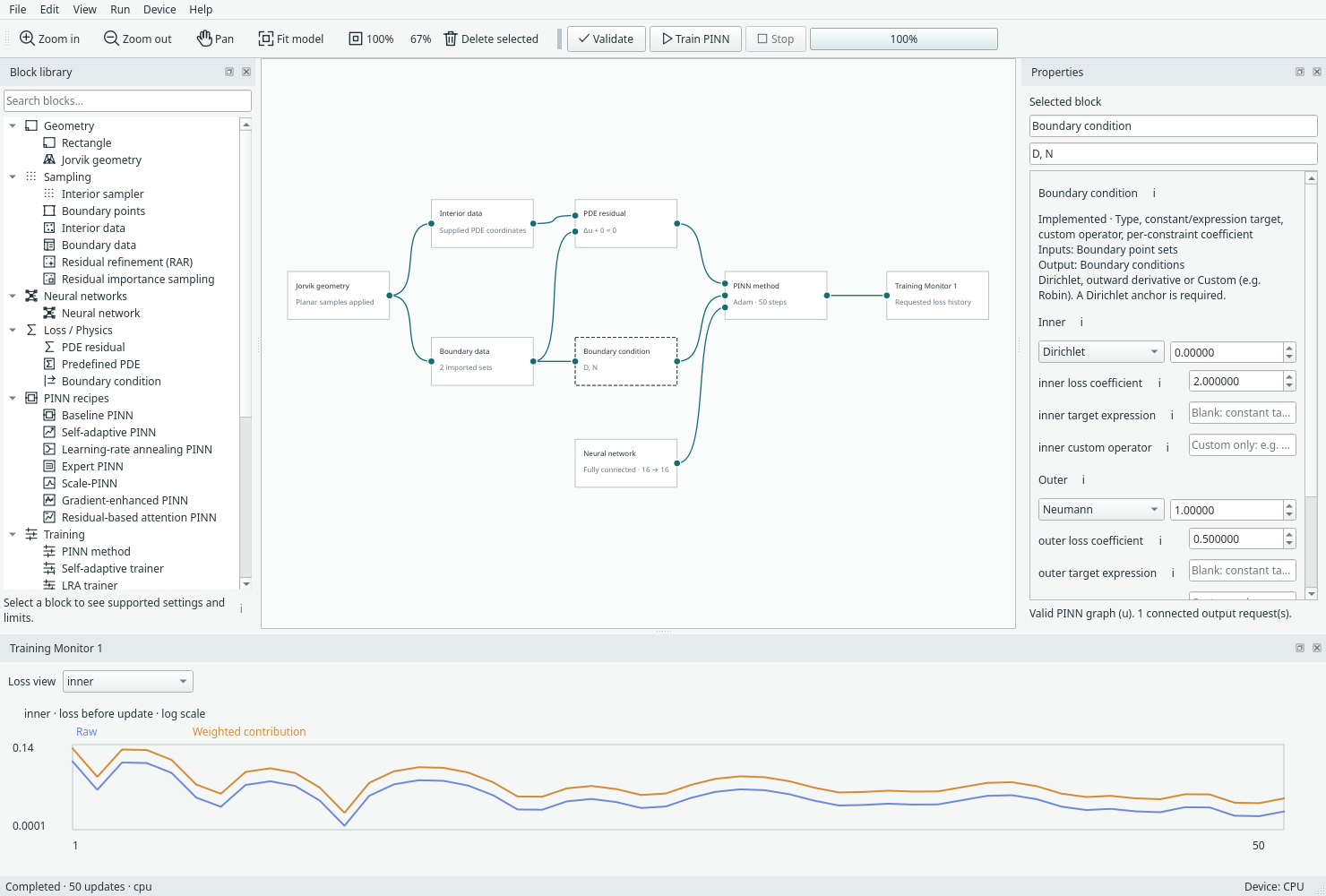
Actual annulus training: inner coefficient 2, outer coefficient 0.5 and overall BC weight 3. The monitor's Loss view selects inner and compares its raw loss with its weighted contribution. This short run demonstrates controls, not accuracy.

Open a connected Training Monitor and choose a named constraint in Loss view. Summary (all losses) restores the existing overview. The selected view plots raw loss and its contribution to the actual training objective, including adaptive mask/EMA weights where applicable. Both are measured before the optimizer update. Old archives have raw curves but cannot reconstruct missing historical weighted contributions; those gaps are labelled rather than guessed.

Coefficients belong to the BC block and survive undo/redo, save/load and run archives. A coefficient change invalidates cached training state. Updating Jorvik clears coefficients for removed/renamed BC aliases along with their old operator settings; undo restores them. The original imported points are unchanged.