Expert PINN — Margam’s recipe name¶

Expert PINN is Margam’s label for a recipe based on An Expert’s Guide to Training Physics-informed Neural Networks, Sifan Wang, Shyam Sankaran, Hanwen Wang and Paris Perdikaris, arXiv:2308.08468v1 (16 August 2023). The authors do not name a method “Expert PINN”. This is not a mixture-of-experts network or an XPINN domain decomposition. Paper · Authors’ JAX-PI repository.

The supplied PDF v1 is the equation reference. The local JAX-PI checkout was reviewed at revision f944a0cd03c7f35a239955505d83bbdc5a07f831; it contains later research as well as the original pipeline. Its licence restricts reuse of source and modifications. Margam implements the paper mathematics independently: no JAX, Flax, Optax, W&B, upstream source or paper PDF is bundled/required. See community attribution and third-party notes.

Start with the concrete example¶

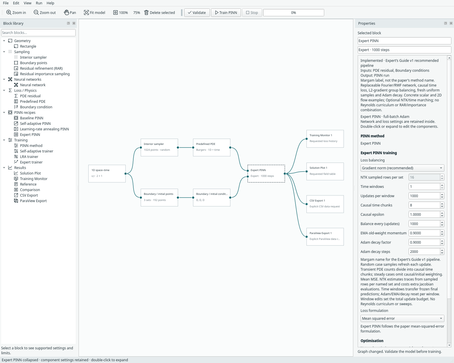
Choose File → Examples → Expert PINN examples → Burgers — Expert PINN · 1D + time. The physics is the existing Burgers initial-value problem, with zero endpoint values and a sine initial profile. Insert Expert PINN for the compact recipe or Expert trainer for an expanded graph. Compact expansion/collapse uses the single definition in margam/recipes/expert.py; the network remains replaceable after expansion.

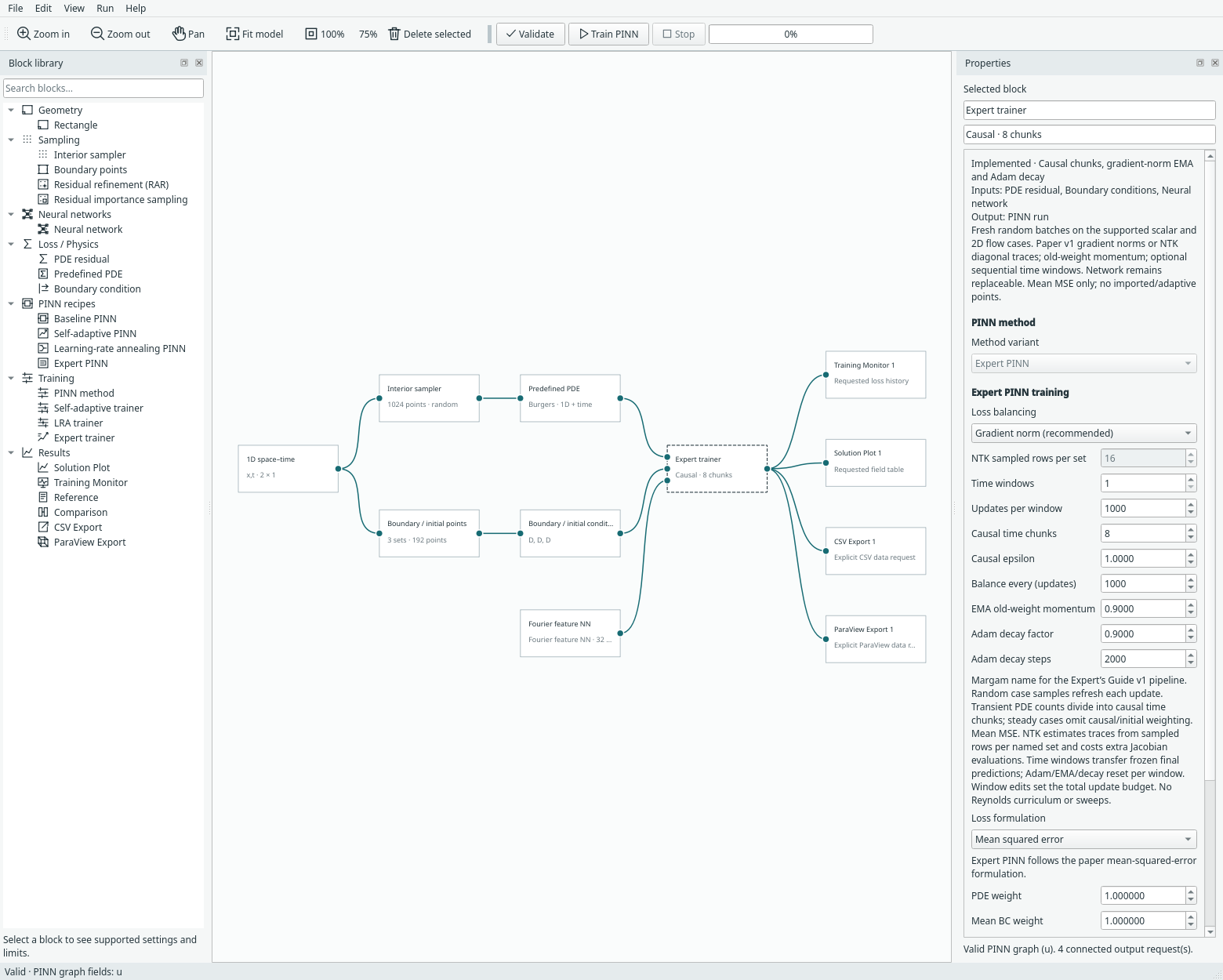
Expert trainer on the existing Burgers physics graph

The seven additional paper examples include steady 2D and 2D space–time workflows, with explicitly labelled initial-field variations.

What this implementation includes¶

Ingredient	Margam implementation
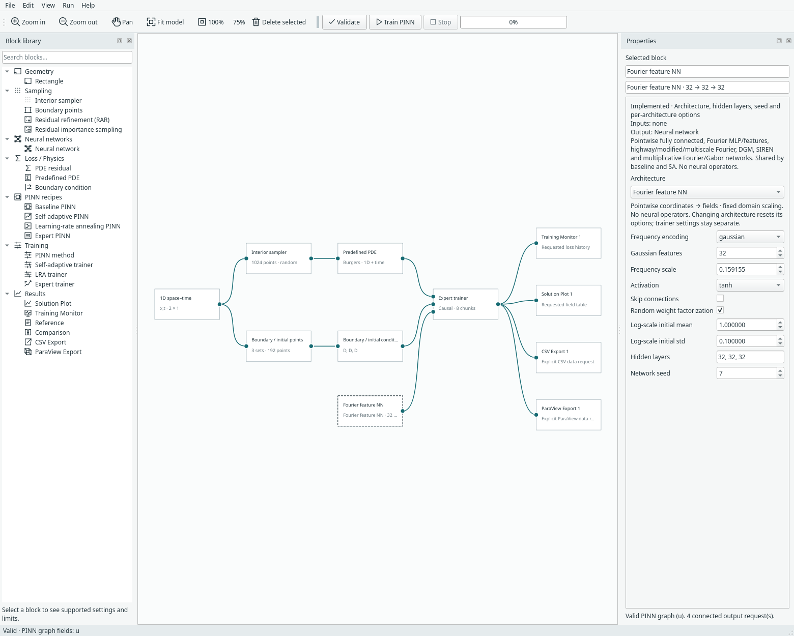
Fourier representation	Existing Gaussian Fourier feature network; default 32 Gaussian vectors and three 32-neuron tanh layers
Random weight factorization (RWF)	Optional exponential per-output-row factors on fully connected, Fourier and modified Fourier networks
Global loss balancing	L2 parameter-gradient norms, sum reference, old-weight EMA; all active groups adapt
Causal residual weighting	Equal-width physical-time strata, detached exponential weights from earlier residual strata
Fresh random training batches	New interior, spatial BC and IC coordinates for every optimiser update; equal interior count per time stratum
Optimisation	Adam, no weight decay, continuous exponential decay of its initial learning rate
Persistence	Coefficients, balancing events, initial data/configuration identity, Adam decay phase and deterministic sampling continuation

Non-dimensionalising the PDE is the user’s modelling responsibility. Fixed network coordinate scaling is not automatic physical non-dimensionalisation. The recipe does not infer physical units or scale PDE coefficients/targets for you.

Random weight factorization¶

For a linear layer with an initialized weight matrix W (PyTorch output rows):

s ~ Normal(mean, std)
V = W / exp(s)[:, None]
W_effective = exp(s)[:, None] * V

Both s and V are trainable; the bias is retained. This follows section 4.3 and Algorithm 2’s exponential parameterization. Initialization preserves the existing network’s effective weights, values and derivatives up to rounding. It is not weight normalisation. Expert defaults use log-scale mean 1 and standard deviation 0.1, including the output layer. Disable/change RWF in the network inspector or replace the network; the Expert trainer does not force an architecture.

The existing Fourier network uses cycles in sin/cos(2*pi*x*B). Expert’s Gaussian scale defaults to 1/(2*pi) for angular scale approximately 1 on the network’s normalized coordinates. It retains the existing raw-coordinate concatenation and frozen feature frequencies. Those are deliberate Margam architecture choices, not exact reconstruction of the authors’ JAX architecture. Disabled RWF preserves existing architecture/checkpoint descriptions.

Reusable RWF controls in the Fourier network inspector

Causal loss — equations (2.10)–(2.11)¶

Split physical time into M equal-width strata and draw the same number of interior samples in each. For stratum mean squared residual L_i:

w_0 = 1
w_i = exp(-epsilon * sum(L_j for j < i))
L_pde = mean_i(w_i * L_i)

w is detached before backpropagation. The first stratum is always active; later strata become active as earlier residuals decrease. Epsilon zero explicitly removes causal suppression. This is weighting within one time slab, not a multi-window marching algorithm. Whole (x,t) pairs stay together: time is never sorted independently and reassigned to unrelated spatial points.

The PDE point count must divide evenly by the causal chunk count. The sampler uses fresh uniform spatial draws and stratified uniform time draws every update. It also refreshes spatial boundary and initial coordinates, preserving their existing types/targets. The connected sampler blocks supply budgets and seeds; select random for all their recipes. Fixed/grid/imported batches are not silently substituted.

Global balancing — equations (2.12)–(2.15)¶

Transient cases have three groups: PDE, initial, and combined spatial boundary loss. Steady cases omit the initial group and causal weighting. Existing static PDE/named-constraint weights are applied before this balancing step; spatial BC contributions are summed into their group. This preserves Margam’s named-set weight convention rather than silently replacing it with a differently pooled BC loss. For each group g, compute its L2 norm n_g over all trainable parameters:

target_g = sum(n_h for every group h) / n_g
lambda_g = momentum * lambda_g + (1-momentum) * target_g
objective = sum(lambda_g * group_loss_g)

Coefficients start at one. Updates occur before steps f, 2f, ..., with default f=1000. Momentum defaults to 0.9 and weights the old coefficient. The causal weights and group coefficients are detached. A norm at/below the configured floor holds its old coefficient; ratios are capped to avoid an unbounded update.

This differs from Margam’s existing LRA trainer: that uses maximum PDE / mean constraint gradient statistics and keeps the PDE coefficient fixed. Do not substitute it for this paper’s all-group L2-norm rule.

Adam decay and diagnostics¶

Before update index k (starting at zero):

learning_rate_k = initial_learning_rate * decay_rate ** (k / decay_steps)

Defaults are initial rate 0.001, decay factor 0.9 and decay steps 2000. These are continuous exponential changes, not staircase changes. The GUI’s existing training update budget remains editable; modest desktop defaults do not reproduce the paper’s benchmark budgets.

The Training Monitor keeps named losses; its PDE curve includes causal weighting but precedes group coefficients. Messages reports learning rate/minimum causal weight at worker progress updates. Right-click the trainer/recipe for Expert training summary, including group coefficients. Closing output views does not stop training.

The same Expert recipe in compact form

Paper versus repository choices¶

Detail	Supplied paper v1 / Margam choice	Reviewed JAX-PI checkout
Balancing numerator	Paper’s sum of group gradient norms	Mean of group gradient norms
EMA parameter	Old-weight fraction, default 0.9	Also old-weight fraction
Balance phase	Before steps divisible by `f`	Burgers loop updates after a network step, starting at loop step zero
Causal partition	Fixed physical-time strata with equally many samples	Sorted random time draws reshaped into equal-count chunks
Weight factors	Paper’s trainable log scales exponentiated in the forward map	Dense implementation initializes positive `g`, then optimizes `g` directly
Burgers boundaries	Existing Margam sine-IC/zero-endpoint case	Reviewed configurations use an exact periodic spatial embedding

The implementations are therefore not claimed numerically equivalent. Exact JAX random-number streams, default architecture, datasets and published accuracy are not reproduced.

NTK and time marching¶

The trainer now offers NTK diagonal balancing and sequential time windows, with frozen initial-field handoff, local optimiser resets and piecewise physical-time outputs. Gradient balancing and one window remain the defaults.

Current limits¶

Expert supports scalar 1D space–time and the concrete steady/2D transient paper examples, with mean MSE. It rejects imported point sets and RAR/importance blocks because its causal strata and per-update sampling policy need an explicit combined design before those can be composed. Use the other supported trainers for those samplers.

Reynolds-number curriculum, automatic physical non-dimensionalisation, exact periodic embeddings, modified JAX MLP architecture, mini-batch gradient accumulation, distributed training and later PirateNet/ActNet methods are not implemented by this recipe. These remain separate extensions.

Model format 18 stores Expert examples and recipe/trainer settings and reads earlier formats. Run archives use restricted tensor/primitive loading. Sampling seeds are derived from the configured seed and update index, and the last active batch is regenerated on resume. Mode/options/physics changes reject resume; iteration budget and device can change. Initial target fingerprints are evaluated canonically on CPU so a GPU archive can be opened for inspection on CPU. Exact continuation is tested on the same device; CPU/GPU floating-point trajectories need not be identical.

Reproduce the software checks¶

python -m examples.expert_pinn --device cpu
python -m examples.expert_pinn --device cuda
python -m unittest discover -s tests -p 'test_expert*.py' -v
python -m examples.capture_expert --overwrite

CPU evidence and CUDA evidence record short 100-update Burgers runs with full settings, finite named losses, balancing events, causal summary, learning-rate decay and exact same-device checkpoint continuation. The smoke configuration uses 128 points, three 16-neuron layers, eight Gaussian features and balancing every ten updates so all mechanisms are exercised quickly. Tests separately verify the formulas, detached causal gradients, RWF derivatives, resampling geometry, coefficient guards, corrupted checkpoints, recipe editing and archives. No shock-reference error or paper-accuracy claim is made.