Original illustrated network walkthrough (dated captures)
Current user manual · Reference catalogue · Network details · Desktop reference · Measured studies
This walkthrough uses an existing interval Poisson example, changes its network to
SIREN, and trains it with SA-PINN. Screenshots are actual Margam widgets captured
on 27 October 2026 from application source e0fde23, light theme, Qt offscreen.
They show implemented controls, not mockups. Shapes and panels may look slightly
different with another desktop/font configuration.
1. Load a complete problem
Start from the repository root:
.venv/bin/python -m margam.ui
Choose File → Examples → 1D examples → Poisson — SA-PINN. This creates
geometry, sampling, PDE, BCs, network, trainer and explicit output/reference blocks.
It solves u_xx + 2 = 0 on [0,1], with zero Dirichlet endpoints and reference
u=x(1-x). No geometry file or mesh is required.
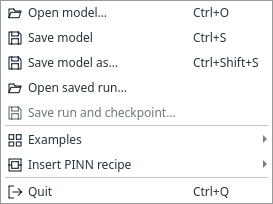
File → Examples loads complete problems; Insert PINN recipe inserts a method's network/trainer construction. Save run is disabled here because no run exists yet.
Loading another example offers Save / Discard / Cancel for unsaved edits. The example wires optional results, but no result window opens automatically.
2. Select a pointwise network
Click the Neural network block. In Properties, open Architecture:
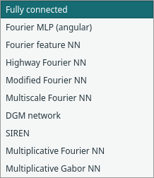
The original fully connected network remains the default. All choices use the same network input on baseline or SA-PINN; these are pointwise networks, not operators.
Changing architecture resets that network's architecture-specific options and is one undoable edit. It does not change the trainer's learning rate or iteration budget. In a compact recipe, double-click the PINN block to expose its network first.
Example: Highway Fourier controls
Selecting Highway Fourier NN exposes its own frequency encoding, frequencies, scale, activation, skip connections and transform/carry switches:
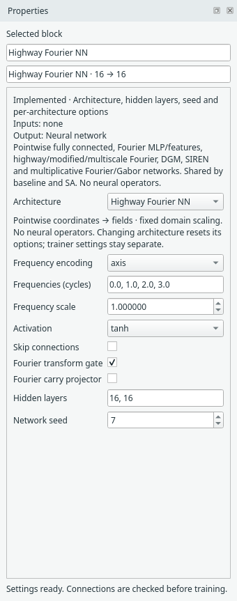
This screenshot shows Highway Fourier's defaults as a controls example. The run below uses SIREN instead. Fourier frequencies are interpreted in normalised domain coordinates. Gaussian encoding replaces the frequency list control with a feature count. See the architecture guide.
Highway/modified Fourier, DGM and multiplicative filters require equal hidden
widths. Skip connections also require equal widths. Use 16,16 or 32,32 rather
than changing only one hidden width for these networks.
3. Configure the SIREN worked example
Choose SIREN, then set its first and hidden omega to 10, keep hidden layers 16,16 and network seed 7:
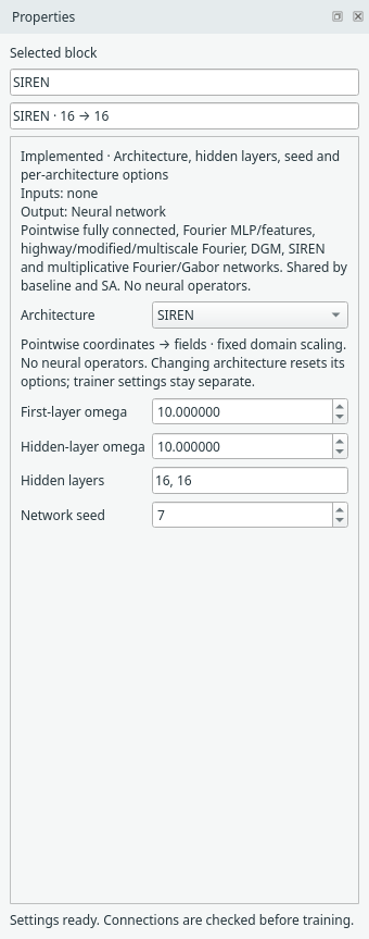
These omega values are deliberate settings for this small smooth problem, not the SIREN UI defaults (both default to 30). The network panel does not own optimiser rates.
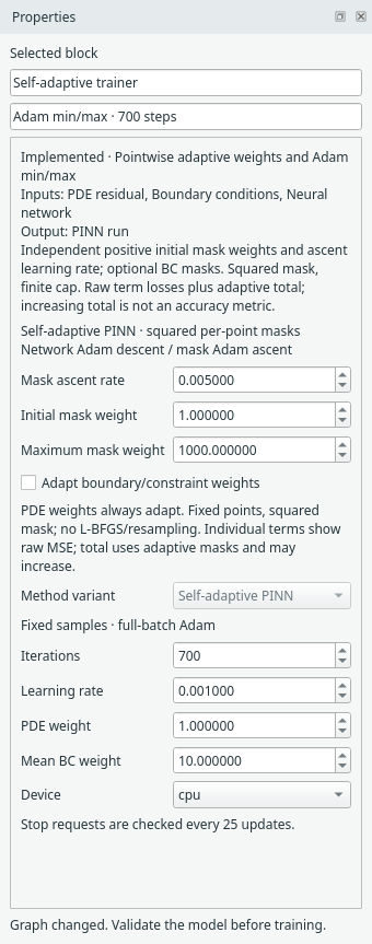
Now select Self-adaptive trainer and configure training separately:
| Owner | Field | Value in this walkthrough |
|---|---|---|
| Domain | Interval bounds | [0,1] |
| Interior sampler | Method / points | Grid / 32 |
| Boundary condition | Left / right | Dirichlet / 0 |
| Neural network | Architecture | SIREN |
| Neural network | First omega / hidden omega | 10 / 10 |
| Neural network | Hidden layers / seed | 16,16 / 7 |
| Self-adaptive trainer | Iterations / network learning rate | 700 / 0.001 |
| Self-adaptive trainer | PDE / mean BC weight | 1 / 10 |
| Self-adaptive trainer | Mask ascent rate / initial λ / maximum λ | 0.005 / 1 / 1000 |
| Self-adaptive trainer | Adapt boundary/constraint weights | Off; PDE masks still adapt |
| Self-adaptive trainer | Device | CPU |
| Comparison | Evaluation points | 201 |
| Reference | Coordinate expression | x*(1-x) |
The example supplies the domain, points, BCs and Reference. Set Comparison's resolution to 201 if following this capture exactly. The capture also uses 201 for Solution Plot and CSV Export; each output owns its own evaluation setting. High-frequency features and sine networks can need different rates/sampling. These values are one demonstrated setup, not a universal preset for every PDE.
4. Understand expanded and compact recipes
Expanded form shows SIREN connected to the SA trainer's network input. Geometry, samplers, PDE, BCs and requested outputs remain outside the recipe:
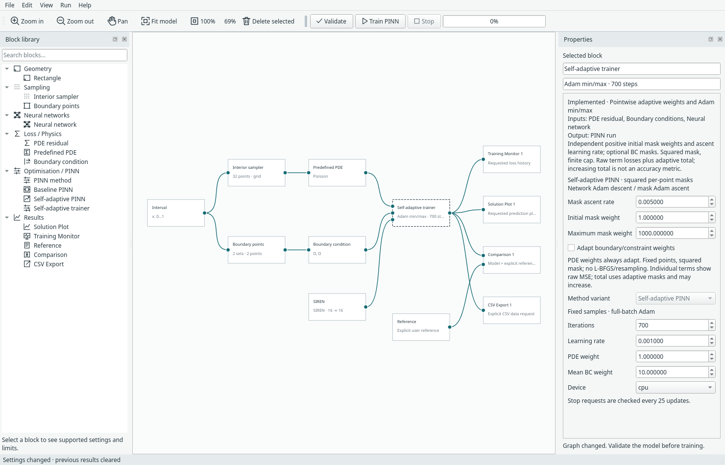
Select SIREN to change its architecture/options. Select the trainer for rates, mask settings and loss weights. Both blocks are constructed from the SA recipe.
Right-click the trainer → Collapse as Self-adaptive PINN:
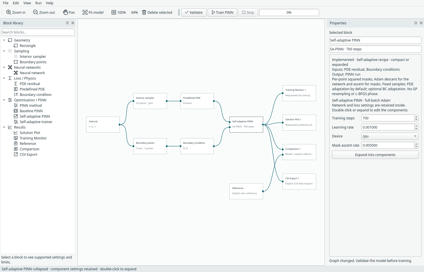
The compact block retains the SIREN architecture, both omegas, widths, seed, training settings and external connections. Its inspector exposes only the recipe's compact controls; it does not turn the hidden network back into FCNN.
Double-click the compact block or use Expand into components to edit the network again. Baseline has the same interaction. A shared network cannot be collapsed; the hard-Dirichlet variant is not relabelled as a baseline recipe.
Do this before training, or save the current run first. Expanding/collapsing is a structural graph edit and clears cached run data, even when the numerical settings are unchanged. Undo restores the earlier graph/layout, not old training results. Recipe details.
5. Train, then explicitly open the monitor
Click Validate, then Train PINN. Progress/status remains available without an open figure. After training, double-click Training Monitor or use its right-click Open monitor action:
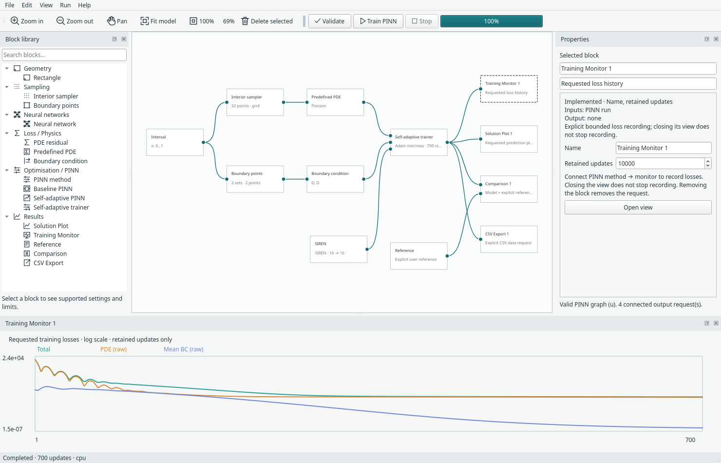
This dock was explicitly opened for the screenshot. It is owned by the monitor block, not a default global results pane. Losses are measured before each update.
The total includes global loss weights and SA's changing λ² masks. PDE and mean BC curves show raw physical MSE. Their sizes and trends cannot be treated as directly comparable unweighted objectives across methods. A rising masked total need not mean worse field accuracy. Closing this view hides it; connected monitoring still retains records up to its configured limit.
For learned λ statistics, right-click the completed SA block → Adaptive weight summary. That reports λ minimum/mean/maximum, not λ². No weight plot is assumed.
6. Compare only when an explicit reference exists
Double-click Comparison. It needs both the trained-model connection and the Reference connection; ordinary Solution Plot does not assume an exact solution.
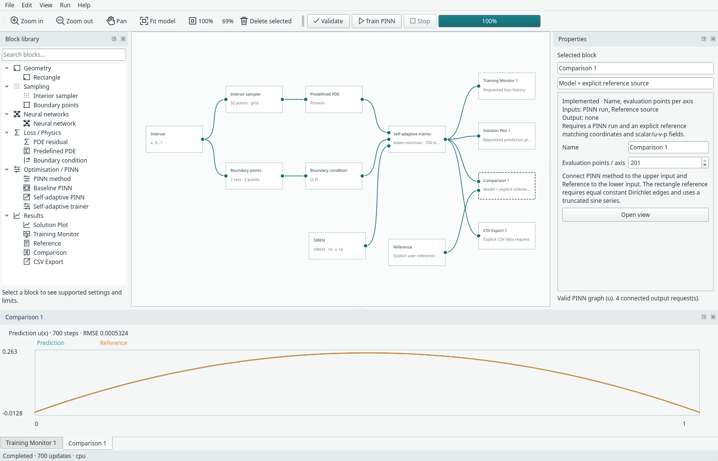
For this actual captured run, the caption reports approximately 5.32×10⁻⁴ RMSE after 700 updates at 201 evaluation points. Prediction and reference nearly overlap; use the metric rather than visual overlap to judge error.
This one CPU illustration is not a new multi-seed study or an architecture ranking. It uses the interval reference, not a rectangular heatmap. For other physics, supply a valid expression/data reference or omit Comparison. The separate twenty-run compatibility study records its full protocol, predictions and limitations. The UI and benchmark paths can differ in their last floating-point digits.
7. Keep the model or the trained run
| What you need | Action | What is saved |
|---|---|---|
| Reopen/edit the construction | File → Save model | .margam.json: graph and settings; no trained state |
| Inspect results or resume later | File → Save run and checkpoint | .margam-run.pt: model, requested results and compatible training state |
| Use prediction rows elsewhere | Connected CSV Export block → Export CSV | Coordinates and predicted fields; no reference/error columns |
Opening a saved run keeps result views closed until requested. SA archives retain both Adam states and masks. Run → Resume checkpoint adds updates on CPU and checks architecture/options, data and optimiser compatibility. Changing architecture or its settings invalidates the current run; save first rather than attempting to resume a different network from the old checkpoint.
Capture provenance and reproduction
Capture manifest records source commit,
theme/platform, image hashes, the complete training configuration and the observed
comparison metric. Application source was unchanged during capture. Personal
layout/recovery files were not read or written (Window(state_directory=False)).
No numerical or plot implementation changed for these screenshots.
To recapture into a new screenshots directory:
.venv/bin/python -m examples.capture_ui_docs --output-dir assets/screenshots/guide-recapture
The helper renders real menus/panels, checks that collapse/expand retains the
configuration, trains the one CPU example, verifies views stayed closed until
requested, and captures the monitor/comparison only after explicitly opening them.
It refuses to replace existing guide captures unless --overwrite is supplied.
It does not create a new environment or change personal UI preferences.