Your first PINN¶

This walkthrough opens a ready-wired 1D Poisson problem, trains it, opens optional results and saves the work. You do not need to draw the graph or import geometry.

1. Open a complete example¶

Choose File → Examples → 1D examples → Poisson — baseline. Save or discard existing unsaved edits if asked. The example opens as a new editable model.

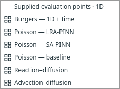
The 1D submenu groups baseline, SA and LRA Poisson with two other scalar examples. Open full size.

The problem is u_xx + 2 = 0 on 0 <= x <= 1, with zero values at the two ends. Its separate Reference block supplies x*(1-x) for the Comparison output. “Interval” in the geometry controls means a 1D line segment, not a time interval.

2. Read the graph¶

Follow the connections: domain → interior points → PDE; domain → boundary points → BCs; network → trainer. The trainer connects to the requested outputs. Click a block to see its settings in Properties on the right.

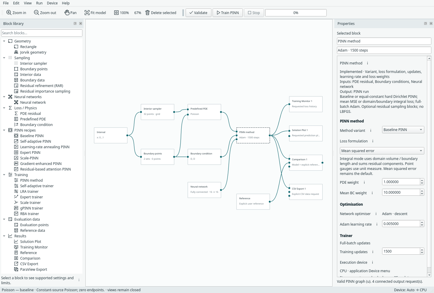
A complete 1D example with separate network and trainer and explicitly connected outputs. Open full size.

3. Find the training controls¶

Select PINN method. Properties separates PINN method, Optimisation and Trainer. The default example uses a fully connected network with 16×16 hidden layers, Adam, and 1,500 updates. You can change these later; use the defaults for this tour.

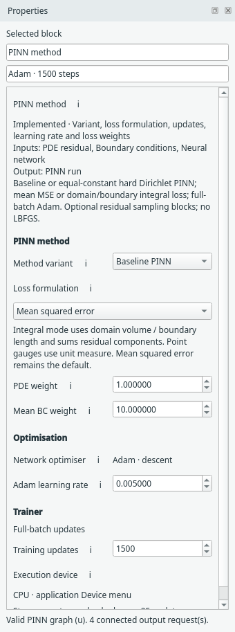
The three settings groups distinguish the method, Adam and the run budget. Open full size.

4. Validate and train¶

Click Validate, then Train PINN or press F5. The progress indicator shows training progress. Editing is locked during the run; canvas navigation remains available. Stop retains a partial run and is checked between batches.

Training does not open figures or write export files. This is intentional.

5. Open the results you requested¶

Double-click Training Monitor to see losses. Double-click Comparison to see predictions alongside the explicitly connected reference. Each view belongs to its output block. Closing or hiding a view does not remove its block.

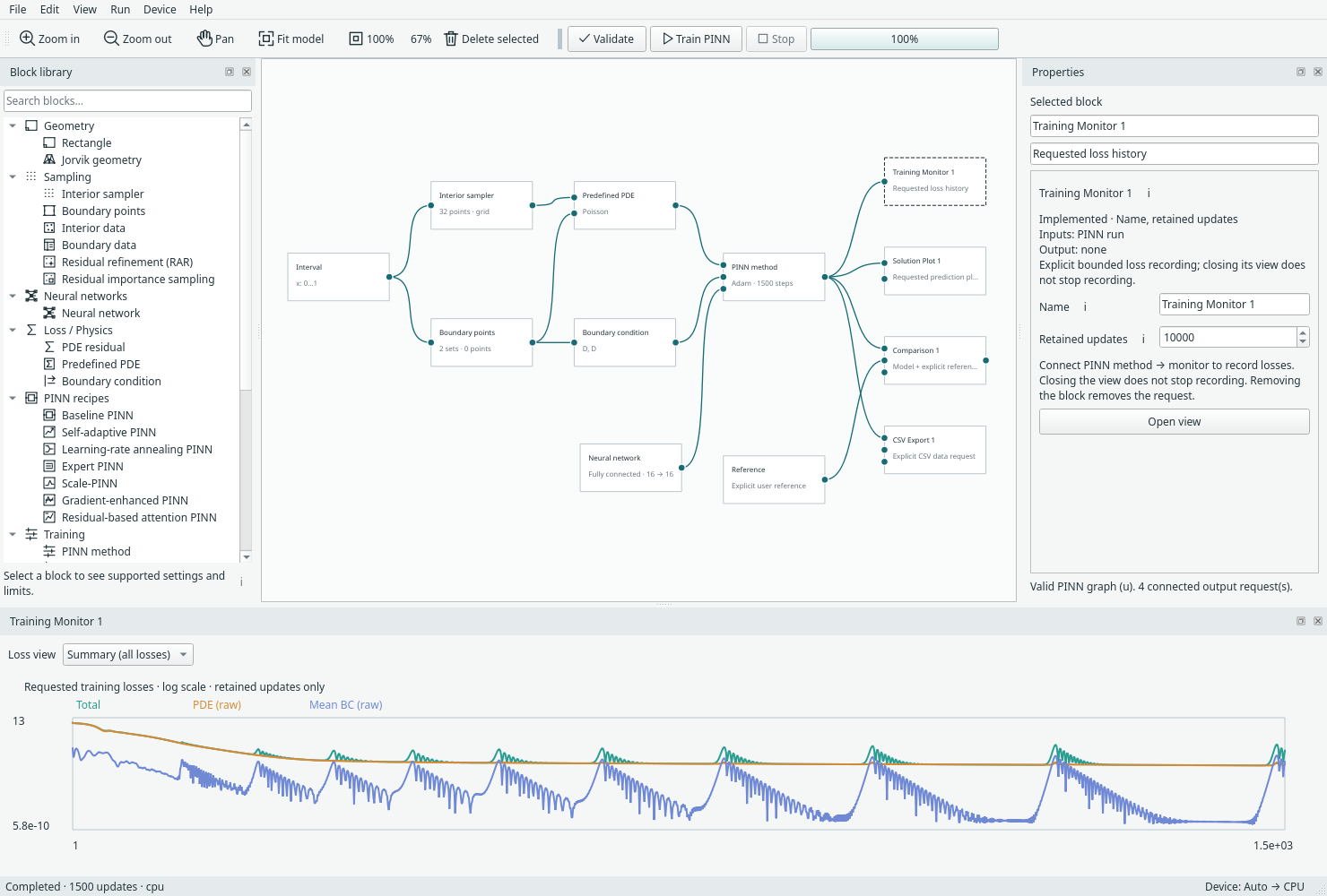
Training Monitor opened explicitly after the default example completed. Open full size.

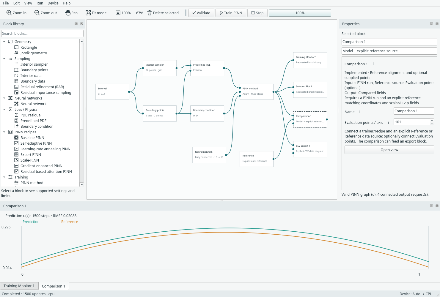
Comparison uses the separate Reference connection; normal prediction outputs do not assume one. Open full size.

The screenshots illustrate where information appears, not an accuracy target. For what each loss curve means, read Training and results.

6. Save the model and the trained run¶

Choose File → Save model as… to save the graph as .margam.json. If you want the trained weights, results and ability to continue, also choose Save run and checkpoint… for a .margam-run.pt file. These files have different jobs.

Next: Learn the workspace, change a network, or save and resume in detail.