Domain and boundary integral loss
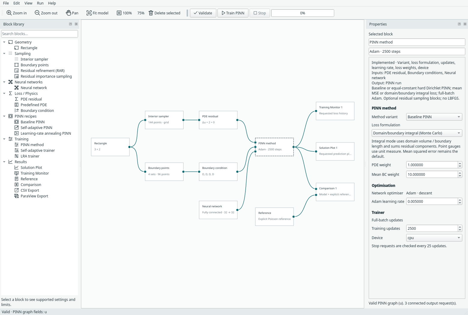
Select a PINN trainer or compact recipe and choose Loss formulation → Domain/boundary integral (Monte Carlo). Mean squared error remains the default, including when opening older models. This option changes loss assembly; it does not change the network architecture or PDE.
Community provenance
This PINN loss formulation follows NVIDIA Modulus / Modulus Sym, subsequently PhysicsNeMo Sym: treat squared pointwise error as a domain/boundary integral and approximate it using sampling weights. The implementation is independently written. See community methods and attribution for sources.
What is integrated?
The PDE term is the integral of its squared residual over the domain. Each BC term integrates its squared error over that named boundary set:
L_pde = integral_domain sum_components(residual_component^2) dV
L_bc  = integral_boundary sum_components(boundary_error_component^2) dS
For N uniformly distributed points in a region of measure V, the Monte Carlo
estimate is V/N * sum_i(sum_components(error_i^2)). Random samples provide
Monte Carlo estimates; cell-centred grids give equal-cell quadrature instead.
Hammersley/stratified methods retain their documented uniform-domain construction.
No random resampling is required to select this formulation.
This follows the area-weighted squared pointwise loss in NVIDIA Modulus / PhysicsNeMo Sym's PointwiseLossNorm, which multiplies point errors by integration weights before summing. Margam's implementation is independent and does not require NVIDIA's package.
It is not the square of the integrated residual: opposite-sign residuals must
not cancel before squaring. NVIDIA's separate IntegralLossNorm applies to a
target on an integrated quantity, for example a total flux. Such integral
constraints are not added by this change. The PDE remains strong-form; this is
not a weak-form/variational PINN.
Measures and vector fields
| Set | Measure used |
|---|---|
| 1D interior | Physical interval length |
| 2D interior | Physical rectangle area |
| Rectangle left/right boundaries | Rectangle height |
| Rectangle bottom/top boundaries | Rectangle width |
| 1D endpoint BC | Unit counting measure per endpoint |
| Pressure gauge | Unit measure: it remains a point penalty |
On a 3 × 2 rectangle, PDE terms scale by 6, vertical-edge terms by 2 and
horizontal-edge terms by 3 compared with scalar mean MSE at the same network.
Point counts do not introduce an extra multiplicative factor.
For coupled PDEs the integral formulation sums squared residual components, matching separate per-field integrals. Mean mode keeps the existing average over components. Therefore changing a vector problem to integral mode changes both geometric measure and component normalisation, even on a unit square.
Global PDE weight, averaged-across-sets BC weight, pressure-gauge weight
and LRA coefficients still apply after term construction. For example the scalar
BC multiplier remains boundary_weight / number_of_sides; selecting integral
mode does not silently remove that existing convention. Larger domains or longer
boundaries can change the loss balance. No automatic physical nondimensionalisation
or weight tuning is performed.
PINN methods and sampling
Baseline, hard-Dirichlet, SA-PINN and LRA trainers support this formulation. SA-PINN applies its squared masks inside the measured loss; monitor term curves show the corresponding unmasked integral estimates. LRA uses gradients of these measured terms for its coefficient updates. Hard-BC errors remain zero by construction.
For Residual importance sampling, with uniform candidate pool size M, draw
probability p_i, and B draws:
L_pde_estimate = V/B * sum_draws(sum_components(error_i^2)/(M*p_i))
The probability correction and volume each appear once. BC sampling stays fixed. The estimate targets the current uniform finite candidate pool; it is not an exact continuous-domain integral. See importance sampling.
RAR is rejected with integral mode. Greedily inserted anchors lack quadrature weights for the uniform domain measure. Multiplying their unweighted mean by volume would not make it an unbiased Monte Carlo estimator. Use mean loss for RAR or choose importance sampling for a corrected integral estimate.
Imported interior/boundary sets are also rejected in integral mode: their region measures and per-point quadrature cannot be inferred reliably from a bounding box. Explicit imported quadrature support belongs to the future GeoSampler data contract.
Save, resume and verification
Model format 14 stores the choice inside trainer/recipe parameters. Earlier model versions default to mean loss. Integral checkpoints record the mode and named measures; resume rejects a different formulation or measure. Mean checkpoints keep the existing format/behaviour. Compact expansion/collapse, undo and archives retain the selection. Geometry and initial-data checks continue to apply.
Reproduce the small CPU workflow check from the repository root:
python -m examples.integral_loss
python -m unittest discover -s tests -p 'test_integral_loss*.py' -v
python -m examples.capture_integral_loss --overwrite
The recorded CPU evidence verifies initial scalar measure scaling on a non-unit rectangle and exact checkpoint continuation with fixed and importance sampling. Tests also cover vector sums, parameter gradients, boundary lengths, endpoint/gauge measures, residual cancellation, all supported trainers and UI persistence. These are software correctness checks, not claims of improved solution accuracy.