Pointwise neural networks for PINNs¶

Documentation index · Illustrated walkthrough · Components · Results

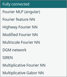
Select a Neural network block and choose Architecture in Properties. The same block/port works with baseline and self-adaptive PINN. No PhysicsNeMo installation or new dependency is needed. Library search for Fourier, DGM, SIREN or Gabor finds the network component; select the architecture in its properties.

Choose and edit a network¶

1. Load a problem from File → Examples. Different examples select their own starting architectures.
2. If the PINN is compact, double-click it to expose the network/trainer pair.
3. Select Neural network → Architecture, then choose the implementation.
4. Edit its own frequency/gate/omega settings and hidden widths/seed. Equal-width restrictions are listed below; changing architecture resets its options.
5. Select the trainer separately for learning rate, update budget and loss/mask settings. Architecture selection does not retune these automatically.
6. Validate/train and open only the connected output views you need. Save the run before changing architecture if you want to retain its weights/results.

The worked example separates SIREN omega controls from the SA trainer controls. For example, omega=10 belongs to the network; lr=0.001 belongs to training. Fourier control screenshot shows the different options for the highway architecture. These screenshots are UI evidence; the measured comparisons and their settings are in results.

Scope and common contract¶

Every supported network maps independent coordinate rows (N,D) to field rows (N,C): D=1 or 2 and C=1 for scalar physics or 3 for steady u/v/p. Domain bounds supply fixed [0,1] coordinate normalisation for the original networks. Affine Fourier NN instead uses physical coordinates by default, with an explicit option to normalize first. Both preserve physical-coordinate chain rules and avoid batch-dependent predictions/derivatives. Seeded initialisation and Fourier/Gabor sampling use Torch's RNG. No batch normalisation, dropout, grid input or dependencies between sample rows are introduced.

These are pointwise networks, including coordinate Fourier features and filters. They are not FNO/AFNO, spectral convolutions, graph/attention operators or learned maps between discretised functions. Those operator architectures were deliberately excluded. DGM here is a network architecture; it does not add a separate DGM sampling/training algorithm. The selected PINN method still owns the physics loss and training procedure.

Implemented architectures¶

Shared smooth layers/scaling are in pointwise.py. factory.py selects the concrete implementation; the Torch-free settings catalogue supplies UI choices and validated serialisation. The original FCNN constructor, parameter names, initialisation and predictions remain bitwise identical at the same seed.

Settings and equations¶

All architectures retain hidden-layer widths and the independent network seed. Use 1–6 hidden layers and 1–256 neurons per layer. Highway/modified Fourier, DGM and multiplicative filters require equal widths (for example 32,32). Skip connections also require equal widths. Other architectures allow unequal widths.

Changing architecture resets its architecture-specific options; trainer settings are unchanged. The change is one undoable edit, so Undo restores the previous architecture and options together. Invalid layer drafts remain editable but cannot train. List controls accept comma-separated finite numbers.

Fourier encodings¶

Standard/highway/modified Fourier use sin(2π x B), cos(2π x B), concatenated with normalised raw coordinates. axis, full Cartesian-product and diagonal encodings use the specified frequency list; gaussian draws a fixed random matrix with configurable feature count and scale. Deterministic encodings also apply the frequency scale. Frequencies are cycles per normalised coordinate, not necessarily cycles per physical metre. Axis/diagonal redundant zero/repeated directions follow the inspected upstream layout.

Defaults: axis frequencies 0,1,2,3, scale 1; Gaussian count 16 when selected. Lists contain 1–16 frequencies within [-64,64]; Gaussian features 1–128; scale 0.001–64. Fourier MLP instead uses angular frequencies scale*exp(linspace(0,π,modes)) without an additional 2π; default 4 modes and scale 1. It generalises the upstream pointwise FourierMLP feature construction to the chosen Margam hidden widths and field readout.

Highway uses T=sigmoid(project_T(features or raw x)), P=project_P(features or raw x) and h = T*activation(W h+b) + (1−T)*P at each hidden stage. The gate uses Fourier features by default; the carry projector uses raw coordinates by default. Both switches are exposed. Modified Fourier uses encoders U,V and hidden state Z with h=U+(V−U)*Z; Z follows the selected smooth activation and is not necessarily a convex mixing coefficient. These are distinct architectures, not aliases.

Multiscale uses independent Gaussian matrices at up to four scales, with one shared MLP and a linear readout of concatenated branch states. Defaults: scales 1,2, 16 features per scale. Smooth tanh (default), SiLU or sine and optional upstream-style skip connections are available for these Fourier networks.

DGM and SIREN¶

DGM forms Z,G,R from coordinate/state affine pairs, forms H using the R-gated state, then updates S=(1−G)*H+Z*S. The configured smooth activation is applied to all four gates, as in the inspected NVIDIA implementation; the default here is tanh, while NVIDIA's inspected full DGM class defaults to sine. Depth is the number of hidden-width entries: one initial layer plus depth−1 gated cells.

SIREN exposes first-layer and hidden-layer omega, both default 30 (range 0.01–100). Its first weight bound is 1/input-width, hidden bound sqrt(6/input-width)/omega, and final linear-layer bound sqrt(6/input-width), following NVIDIA's supplied SirenLayer variant. Biases use ±sqrt(1/input-width). The last layer has no sine. The hidden omega initialisation cancels its activation scale; first omega still strongly influences derivatives. Retune rates/frequencies rather than assuming FCNN training defaults suit every SIREN problem.

Multiplicative filters and explicit adaptations¶

Filter frequencies/phases are learned network parameters. Input scale (default 1) is divided by sqrt(depth+1); each stage multiplies an affine state by a fresh coordinate filter. There are depth+1 filters and depth affine mixing stages. Gabor adds centres and Gamma-initialised widths (shape 6, rate 1 by default). Widths use a softplus parameterisation to stay positive. Squared distance is computed directly as a sum of squares, avoiding the undefined second derivative of a norm at a filter centre. These two changes from upstream are intentional for PINN Hessians. Tests include evaluation exactly at a Gabor centre.

No weight normalisation, learned activation parameters, dictionary/key wrappers, parameter-input encodings or upstream normalisation framework was imported. Margam uses small defaults, fixed domain scaling, its own field contract and explicit settings; this is an adaptation, not upstream checkpoint/config compatibility.

Recipes, models and checkpoints¶

Baseline and SA recipes share the architecture setting. Expand a compact recipe to choose/edit its network, then collapse its trainer to retain the complete architecture and option dictionary. Individual network blocks remain replaceable through the existing typed network input. Examples still default to FCNN unless explicitly configured otherwise; architecture changes do not silently retune rates.

Model format 10 reads formats 1–9 and migrates older network/compact records to FCNN with empty options. New run checkpoints include a network specification (type, canonical options, widths, dimensions, bounds and seed), in addition to weights/buffers and optimiser state. Resume rejects changed settings even when parameter shapes match, such as changed SIREN omega or a same-sized Fourier basis. Earlier FCNN checkpoints without that specification remain supported; new architectures require it. Run archives remain format 2 and use restricted loading.

Use from Python¶

from margam.templates.poisson import PoissonConfig, build_pinn

config = PoissonConfig(shape='Interval', points=32, layers=(16,16),
                       network_type='siren',
                       network_options={'first_omega':10., 'omega':10.},
                       method='self_adaptive', lr=.001, boundary_weight=10.)
model = build_pinn(config)
model.train(700, display_every=0)

To obtain only the network, use margam.nn.factory.build_network(config); the selected field contract supplies its input/output dimensions. Direct classes live in the files above. Neural-operator type strings and unknown/unsafe settings are rejected, not dynamically imported or executed.

Verification and evidence¶

Network tests check first/second derivatives against numerical differentiation in float64, output shape, per-row independence, Fourier basis and physical-coordinate scaling, gating equations, positive/smooth Gabor behaviour, original FCNN identity, exact checkpoint resume and setting-mismatch rejection. Real u/v/p training is exercised for every architecture with baseline and SA, plus hard-Dirichlet wrapping of DGM. UI tests exercise every architecture through selection, compact/expanded conversion, clipboard, model/run save/open and resume. No result views open automatically.

A recorded compatibility study trains all ten choices with both methods on one small Poisson problem. It uses explicit low-frequency options and a lower SIREN rate, not all UI defaults; parameter counts also differ. It establishes working cases, not universal accuracy or a ranking. High frequencies amplify PDE derivatives and can require different sampling/rates. Current evidence is CPU-only; stiff/multiscale benchmarks and CUDA remain unverified.

Source provenance/licences: THIRD_PARTY.md. Local layer revision 96b7cd1…; full PhysicsNeMo Sym models at 0c5f18c…. These sources were inspected and adapted; the original checkouts were not modified.

Random weight factorization¶

Fully connected, Fourier feature and modified Fourier networks expose optional Random weight factorization with log-scale mean/std controls. It preserves the initialized effective function and trains exponential row scales plus direction weights. Existing disabled settings preserve checkpoint architecture descriptions. The Expert PINN guide explains its paper reference, initialization and derivative checks. This is reusable outside the Expert recipe and is not a new neural-operator architecture.

Affine Fourier NN¶

The additional affine_fourier architecture applies explicit affine coordinate expressions, a trainable dense projection and sine features before its shared trunk. Unlike the existing fixed Gaussian features, both projection weights and bias optimize with the network. Physical coordinates are the default; optional normalization is explicit. See settings, example equations and limits.