NTK balancing and time marching
These options belong to the existing Expert trainer and Expert PINN recipe. They implement two distinct ideas from An Expert’s Guide to Training Physics-informed Neural Networks, v1: NTK weighting (equations 5.4–5.9) and sequential time windows (section 5.3). The default remains gradient-norm balancing on one time window. No Reynolds curriculum, grid search or parameter sweep is added.
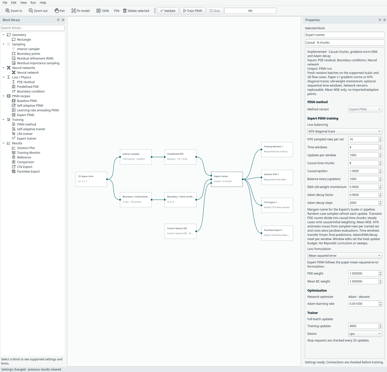
Choose loss balancing
Select the trainer, then choose Loss balancing → NTK diagonal trace. This works on the existing Expert scalar/transient and steady flow examples. Choose Gradient norm (recommended) to retain the original implementation; the paper recommends it as the less expensive first choice.
For each scalar output of a constraint or PDE residual, Margam evaluates the parameter Jacobian gᵢ=∂fᵢ/∂θ. The corresponding NTK diagonal is gᵢ·gᵢ; summing these entries gives its trace. PDE, initial and combined boundary traces are Tᵣ, Tᵢ, Tᵦ. Steady cases omit Tᵢ. The target coefficient for group j is λ̂ⱼ=(Σₖ Tₖ)/Tⱼ, followed by the same old-weight EMA used by gradient balancing.
This differentiates pointwise residuals/constraint operators, not squared losses. A perfectly fitted point can have a nonzero NTK diagonal even though its loss gradient vanishes. Vector components each contribute a diagonal entry; periodic/derivative boundary operators are differentiated as configured. The trace uses unweighted operators, before causal weights and manual loss factors. Existing manual factors still apply to the training objective.
Margam never constructs the full NTK matrix. NTK sampled rows per set caps the rows used from each named condition/PDE set. A seeded random subset without replacement selects from that update's fresh random batch; the sampled diagonal sum is multiplied by full-row-count/sample-row-count. This is an unbiased sampled-row trace estimate when the cap is smaller than a set, and the full diagonal trace otherwise. It is not a random-vector/Hutchinson estimator. It is not divided by the number of rows.
The default cap is 16, with an allowed range of 1–256. Balancing runs at Balance
every (updates). Zero/small traces retain the previous coefficient; the existing
numerical floor and coefficient cap prevent undefined ratios. Non-finite
Jacobians stop the update. The saved balance history's norms entries mean
NTK traces in this mode; the saved configuration identifies which mode was
used. NTK can be substantially more expensive, especially with high-order PDEs.
Train successive time windows
Choose a transient example under File → Examples → Expert PINN examples. Set Time windows above one and set Updates per window. Window edits set Training updates to their product. For example, four windows with 1,000 updates each request 4,000 total updates. There are at most 32 equal physical-time windows and the configured schedule cannot exceed 100,000 updates.
Each window keeps causal strata and its selected balancing scheme:
- The first window uses the problem's supplied initial condition.
- Freeze its final network. At the next window's initial points, evaluate that frozen network at the shared physical time to obtain detached targets.
- Warm-start the next network's trainable parameters. Retain its new local coordinate bounds; reset Adam, loss-balancing coefficients/history and decay phase for the new window.
- Repeat until the final window is trained.
For velocity/pressure cylinder flow, only velocity is transferred as initial data; pressure remains determined by the PDE and traction condition. Torus transfers u/v/vorticity. The cylinder inlet ramp retains its original global-time origin rather than restarting in every window. Spatial BCs and PDE coefficients remain the problem's specified ones. Handoff error can accumulate; the interface initial condition is a soft training constraint, not an exact continuity guarantee.
Gradient balancing and NTK both work with time marching. Single-window steady training remains available, but multiple windows are rejected for steady cases. This is sequential time decomposition, independent of Reynolds curriculum or parameter sweeps.
Results, stop and resume
The monitor counts total updates; the log and Expert summary show the current window and its local update. Training updates is the job's total update budget, whereas Updates per window fixes the transition schedule. If the job stops before the final window has started, no full-domain prediction/export is produced. The checkpoint and loss histories are retained for resume. The log explains that full-domain outputs are being held. Direct prediction beyond the active window's physical end is rejected.
After the last window starts, tables/CSV/ParaView requests evaluate each physical time with its corresponding frozen or active network. An interface timestamp uses the preceding window's final prediction. Time remains a physical coordinate, not an epoch number. PVD playback therefore follows the original full time axis. Resuming after the final window adds updates to that final window; it does not rewrite earlier windows or alter the partition.
Archives store completed windows, the active network/Adam state, all named loss histories and the immutable schedule. Loading reconstructs the teacher chain and validates each window before replacing the live run. Changed schedules, inconsistent phases/history or changed teacher identity are rejected. CPU continuation is tested bitwise at either side of a window boundary. CUDA Jacobian/backward execution can introduce float32 round-off after reopening; the recorded GPU runs compare losses and network tensors with rtol=1e−5, atol=1e−7 and report actual maximum differences. Bitwise identity is recorded separately and is not promised for every GPU configuration or CPU-to-CUDA continuation. Model format 18 migrates older settings to gradient balancing and one window; prior Expert checkpoints remain supported with those defaults.
Run and inspect evidence
python -m examples.expert_extensions --device cpu
python -m examples.expert_extensions --device cuda
python -m unittest tests.test_expert_extensions -v
python -m examples.capture_expert_extensions --overwrite
CPU evidence and CUDA evidence record short training, balancing events and checkpoint continuation with explicit CPU/GPU comparison criteria. These are software correctness checks, not published accuracy reproduction. The implementation is independent paper-based PyTorch code; no JAX-PI source or datasets were copied. See community attribution.