Expert PINN examples
Open File → Examples → Expert PINN examples. All seven problems from the paper's results section are available, alongside the existing Expert Burgers example. Each creates an editable component graph with an independent network, Expert trainer, named constraints and optional output blocks. No output window opens automatically and training writes no export files.
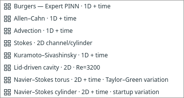
These are independent PyTorch implementations of the equations in An Expert’s Guide to Training Physics-informed Neural Networks, v1. “Expert PINN” is Margam's recipe label. No upstream JAX source or datasets are bundled. See method details and attribution.
Choose a problem
| Example | Space and time | Equation and defaults | Conditions |
|---|---|---|---|
| Allen–Cahn | x ∈ [−1,1], t ∈ [0,1] | uₜ − 0.0001uₓₓ + 5(u³−u)=0 | Initial x²cos(πx); periodic u and uₓ |
| Advection | x ∈ [0,2π], t ∈ [0,1] | uₜ + 50uₓ=0 | Initial sin(x); periodic u |
| Kuramoto–Sivashinsky | x ∈ [0,2π], t ∈ [0,1] | uₜ + αuuₓ + βuₓₓ + γuₓₓₓₓ=0; α=100/16, β=100/16², γ=100/16⁴ | Initial cos(x)(1+sin(x)); periodic u and first three spatial derivatives |
| Stokes channel/cylinder | 2D channel [0,2.2]×[0,0.41], disk removed | −νΔ(u,v)+∇p=0, uₓ+vᵧ=0; ν=0.001 | Parabolic inlet peak 0.3; stationary walls/cylinder; zero outlet traction |
| Lid-driven cavity | 2D unit square, steady | (u,v)·∇(u,v)+∇p−νΔ(u,v)=0, uₓ+vᵧ=0; ν=1/3200 | Top velocity (1,0); other walls (0,0); p(0,0)=0 |
| Navier–Stokes torus — Taylor–Green variation | Periodic 2D square [0,2π]², t ∈ [0,10] | ωₜ+uωₓ+vωᵧ−0.01Δω=0; div=0; ω=vₓ−uᵧ | Self-contained Taylor–Green initial velocity/vorticity; periodic fields and first two normal derivatives |
| Navier–Stokes cylinder — startup variation | Same 2D channel/disk, t ∈ [0,1] | (u,v)ₜ+(u,v)·∇(u,v)+∇p−0.001Δ(u,v)=0; div=0 | Quiescent initial velocity; parabolic inlet peak 1.5 with startup ramp; no slip; zero outlet traction |
Both cylinder cases remove a circle centred at (0.2,0.2), radius 0.05. The domain inspector exposes these values; the disk must lie strictly inside the channel. Uniform rejection sampling excludes the disk. Separate circle samples lie on its surface. Inlet/outlet and wall samples exclude corner intersections.
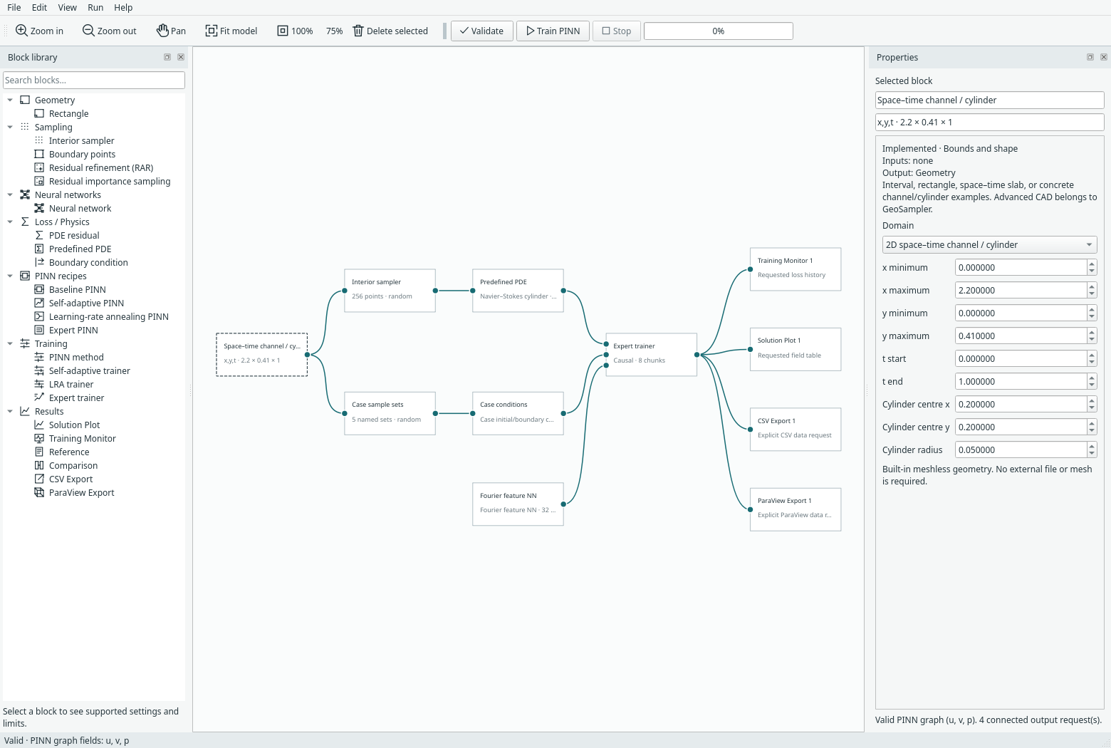
The Stokes equations use dimensional coordinates/coefficients rather than the paper's nondimensional L=0.1, U=0.2 form. Outlet traction at the right edge is (νuₓ−p, νvₓ)=0. It fixes pressure level, so these cases do not add a pressure gauge. The cavity does require one gauge. Its moving-lid corner discontinuities are preserved: boundary sampling omits the corners rather than smoothing the lid.
Explicit variations
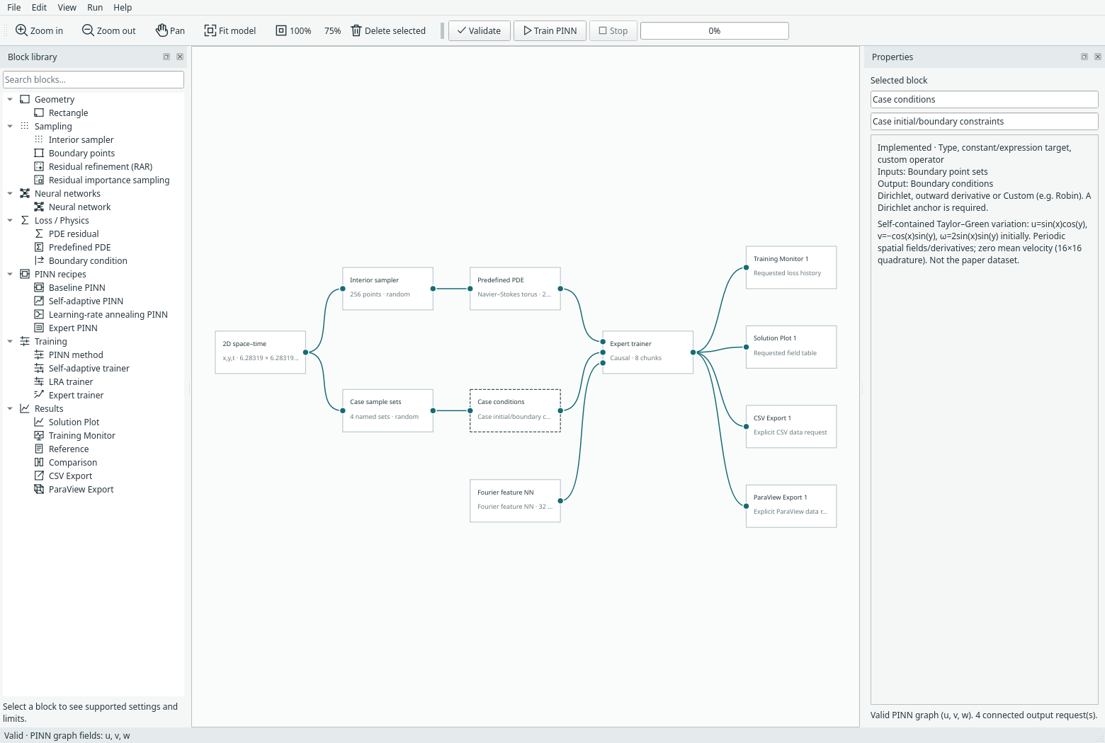
Torus: this means a periodic planar domain, not a 3D surface. The original experiment's externally supplied initial field is replaced with u₀=sin(x)cos(y), v₀=−cos(x)sin(y), ω₀=2sin(x)sin(y). The network predicts three outputs u, v, w, where w means scalar vorticity ω, not a third velocity. A curl-closure residual ties w to vₓ−uᵧ; this auxiliary-field representation differs from differentiating velocity to obtain every vorticity prediction. Its PDE and initial/periodic constraints are all trained explicitly. A zero-spatial-mean velocity constraint removes the time-dependent uniform drift left undetermined by curl/div equations. It uses a 16×16 periodic quadrature at up to eight sampled times per update; this is a soft quadrature constraint, not an exact projection. The chosen Taylor–Green initial velocity has zero mean.
Transient cylinder: the paper uses an initial field obtained from a prior flow simulation. Margam starts with u=v=0 and ramps the parabolic inlet by 1−exp(−(t−t₀)/τ), τ=0.1. Pressure has no prescribed initial value. This startup case is deliberately labelled a variation and does not reproduce the paper's wake.
Training and outputs
The default recipe uses Gaussian Fourier features with optional random weight factorization. Replace the network after expanding a compact recipe, or edit it in the expanded example. These cases support Expert or baseline training; SA/LRA, imported geometry, RAR/importance sampling and integral loss are rejected for these new contracts until their transfer/quadrature rules are implemented.
Expert training refreshes interior/condition points every update. Transient interiors use equal physical-time strata and detached causal weighting. Steady cases balance two groups (PDE/boundary), without causal weighting; transient cases balance PDE/initial/boundary. Periodicity is a soft loss, not an exact periodic network embedding. Allen–Cahn uses the classical initial profile, whose endpoint derivative mismatch is handled as an initial/periodic loss, not forced corner data.
The default is one time slab; optional time marching and NTK balancing are available in the Expert trainer. There is no Reynolds-number curriculum for the cavity. Default small networks/sample counts are usable starting graphs, not the paper's training configurations or accuracy results. No later-time analytical reference is assumed or added automatically.
Solution tables and CSV preserve coordinate/field names. ParaView Export is an explicit connected block: right-click it after training to write a file. Steady rectangular fields use VTI; steady obstacle fields use VTU vertex point clouds. Time-dependent examples use PVD collections with physical-time VTI/VTU frames. The cylinder solid is excluded from both evaluation and export. VTU contains vertices only, no FEM cells or mesh connectivity. The velocity vector is (u,v,0); torus w is a separate scalar vorticity array. See export formats.
Resolution means points per coordinate axis, including time. A 2D transient request with resolution N can evaluate N³ locations before obstacle exclusion. Requests above 100,000 locations are rejected; the default for these cases is 9. Higher resolution does not retrain the network.
Recorded correctness checks
The CPU record and CUDA record contain complete small configurations, named sample counts, ten updates of finite losses and exact same-device checkpoint continuation for each case. They make no convergence or solution-accuracy claim. Automated checks additionally compare manufactured PDE residuals, periodic derivatives through third order, obstacle sampling, physical-time exports, UI worker execution, compact graphs and run archives.
python -m examples.expert_suite --device cpu
python -m examples.expert_suite --device cuda
python -m unittest tests.test_expert_examples -v
python -m examples.capture_expert_suite --overwrite