Residual-based attention PINN
Choose File → Examples → RBA examples for Allen–Cahn or 2D Helmholtz. Residual-based attention PINN is also a compact recipe under PINN recipes, with a separate RBA trainer under Training. The network remains replaceable.
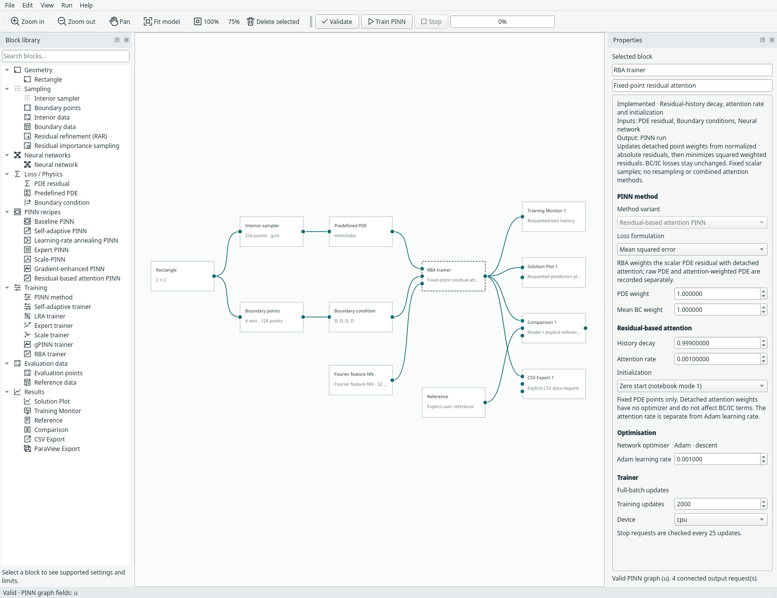
RBA attention settings are separate from Adam learning rate and network settings. Open full size.
RBA here means pointwise residual weighting, not Transformer self-attention. There are no queries/keys/values and no extra attention network or optimizer. It follows Anagnostopoulos, Toscano, Stergiopulos and Karniadakis, Residual-based attention in physics-informed neural networks, with verification against the authors' code.
The update rule
For each fixed scalar PDE point, compute its physical residual error r, including its PDE target. Before the network update:
q = abs(r) / max(abs(r))
lambda_next = gamma*lambda + eta*q
L_PDE_attention = mean((stop_gradient(lambda_next)*r)²)
L_total = w_PDE*L_PDE_attention + sum_j w_j*L_BC_or_IC_j
The maximum is over the fixed PDE point set. If every residual is zero, q is explicitly zero, avoiding a 0/0 division. The old attention then decays normally. The weight multiplies the residual before squaring; this is not mean(λr²). Normalization, recurrence and attention weights are detached from autograd. Gradients still flow through r into the network parameters.
Boundary/initial-condition operators and losses are unchanged. Attention applies to PDE rows only. The same point retains its accumulated history at every update. The candidate mask is committed only after finite-loss/gradient checks and the successful optimizer step. Validation, inspection and output evaluation do not advance attention.
Controls and initialization
| Control | Meaning | Default |
|---|---|---|
| History decay | γ, retained contribution of previous attention | 0.999 |
| Attention rate | η, residual-history increment; separate from Adam rate | 0.001 |
| Initialization | First-step attention rule | Zero start (mode 1) |
Both notebook modes are available:
- Zero start: λ starts at zero; the first increment is ηq.
- Normalized first residual: λ starts at zero, but the first increment is q rather than ηq. Later increments use ηq. This reproduces notebook mode 2.
There is no arbitrary mask clamp. For normalized residuals in [0,1], the recurrence's asymptotic scale is η/(1−γ). A normalized first step can temporarily exceed that scale; its global envelope also includes the initial maximum one. The checkpoint validator allows conservative floating-point tolerance around the bound, checks finite nonnegative values and exact row count, and requires zero masks for an untrained checkpoint.
Decay must be between 0 and 0.999999 and attention rate between 10⁻⁸ and 1000. These numeric limits keep the controls finite and γ representable below one in the supported float32 workflow. They are not tuned performance recommendations.
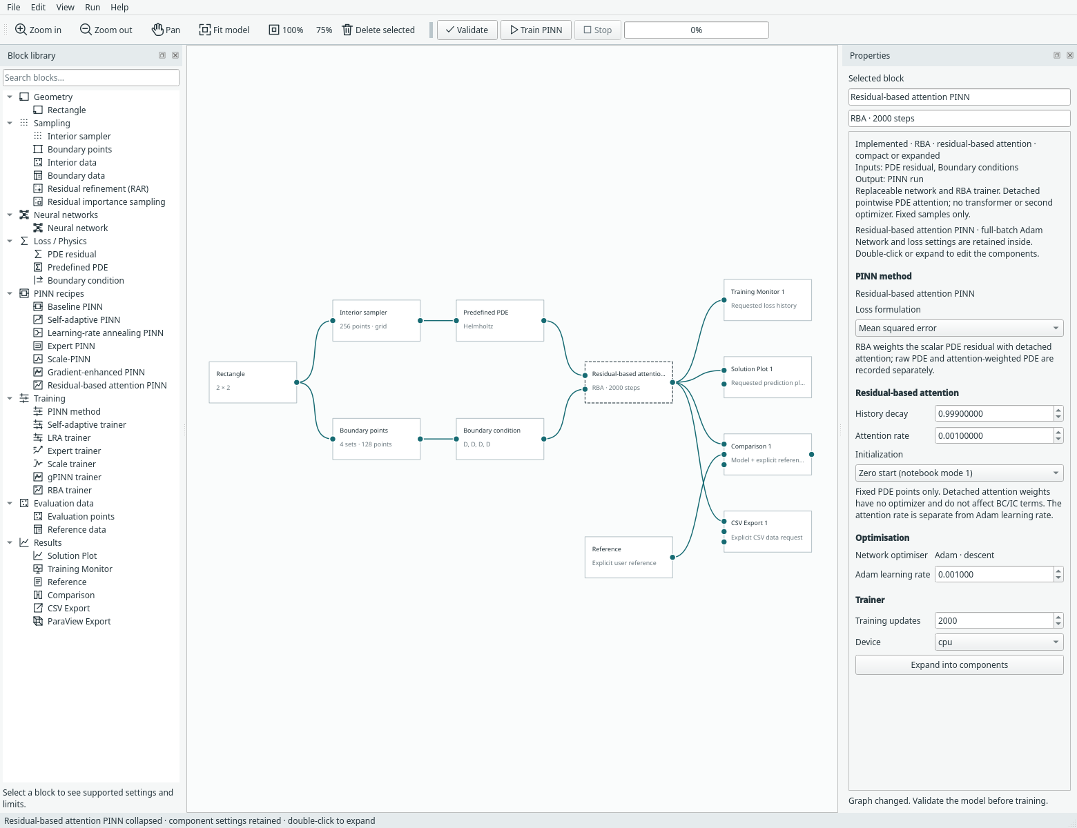
The single definition in margam/recipes/residual_attention.py supplies both
representations. Expand it to replace the neural network; attention stays with
the trainer.
Monitor raw and weighted losses
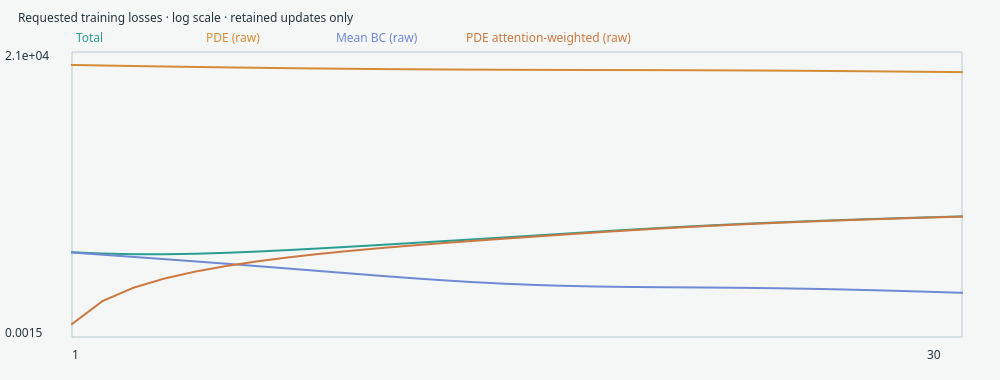
The monitor separately records:
pde: ordinary, unweighted physical PDE MSE.pde_weighted: attention-weighted PDE MSE, before global PDE weight.- Existing boundary/initial terms, unchanged by attention.
total: the actual weighted training objective.
Early in zero-start training, pde_weighted can be very small because attention
has not accumulated yet. It is not evidence of a small physical residual or a
more accurate solution. Raw and attention-weighted curves can move differently.
The trainer/compact recipe's right-click Attention statistics shows the saved
step and mask minimum/mean/maximum; the asymptotic scale is also shown.
These statistics remain available after reopening a run.
Included examples and differences
Allen–Cahn · 1D + time reuses Margam's existing equation, x²cos(πx) initial profile and periodic field/first-derivative constraints on x∈[−1,1], t∈[0,1]. It uses a replaceable fully connected network and fixed random collocation points. There is no final-time constraint and no assumed exact later-time reference.
Helmholtz · 2D reuses the existing sine-forced problem on [−1,1]², with u=sin(πx)sin(4πy) as an explicitly connected reference and the existing Fourier network. The second coordinate is spatial y, not physical time.
These are starting examples for the RBA algorithm, not paper reproductions. Margam retains its own point budgets, network controls, soft initial/boundary constraints, mean-loss grouping and fixed Adam learning rate. The upstream hard transforms, enhanced architectures, learning-rate schedule, datasets and reported accuracy/speedups are not bundled or claimed. Existing heatmaps are not expanded; views/files remain explicit requests.
Fixed-point and checkpoint contract
The first implementation supports scalar interval/rectangle/1D space–time models, prepared 2D scalar data and the concrete Allen–Cahn case. Integral quadrature, RAR/importance resampling, minibatches, coupled/vector residual weighting, inverse parameters and combinations with SA/LRA/gPINN/Scale/Expert time marching are not silently enabled. Moving attention requires a separate transfer contract.
Training rejects changed compiled points/targets, including a reordered point set. Actual resume reconstructs and fingerprints ordered data, normals and targets. Checkpoints retain the detached mask, RBA settings/configuration, network/Adam state and raw/weighted loss history. Changed data, mask counts or attention settings are rejected. Canonical CPU target fingerprints allow GPU checkpoints to validate and resume on CPU; cross-device training is not claimed bitwise identical.
Model format 23 adds RBA settings and reads formats 1–22. Existing methods migrate the unused defaults without changing their losses. Archived predictions can be viewed/exported without original files, while actual training resume needs its source data. Masks belong to training points, not independent evaluation locations; result exports do not invent attention values at new points.
Reproduce the checks
From the repository root using its existing environment:
python -m examples.rba --device cpu --steps 6 --output /tmp/rba-cpu.json
python -m examples.rba --device cuda --steps 6 --output /tmp/rba-cuda.json
python -m unittest tests.test_rba tests.test_rba_ui -v
python -m examples.capture_rba --overwrite
CPU and CUDA records cover both initialization modes on both examples, six updates, detached masks, raw/weighted losses, identical same-device continuation and requested field evaluation. These are software checks, not tuned accuracy experiments. Tests also verify the recurrence and squared-weight derivative analytically, zero-residual handling, failed-step mask atomicity, all network choices, reordered-point/corrupt-mask rejection, older method migrations, UI persistence, CPU loading of GPU archives and Allen–Cahn physical-time PVD export.
The source record stores paper/notebook hashes and the inspected MIT-licensed upstream revision. No upstream code/data is copied into the independent implementation. The capture manifest identifies the actual isolated desktop screenshots.